

Ascertainment of Ecological Footprint …
85
hypothesis as H 1 = long-run coefficients (e.g., a 1 = a 6 0, F − stat bounds ). The Fstatistics is compared with the critical values of lower and upper bounds. If the F-stats
is greater, lesser, or in between the values of lower (I (0)) and upper (I (1)) bounds,
the result is read as cointegrated, non-cointegrated, or inconclusive, respectively.
4 Empirical Results and Discussion
4.1 Descriptive Statistics
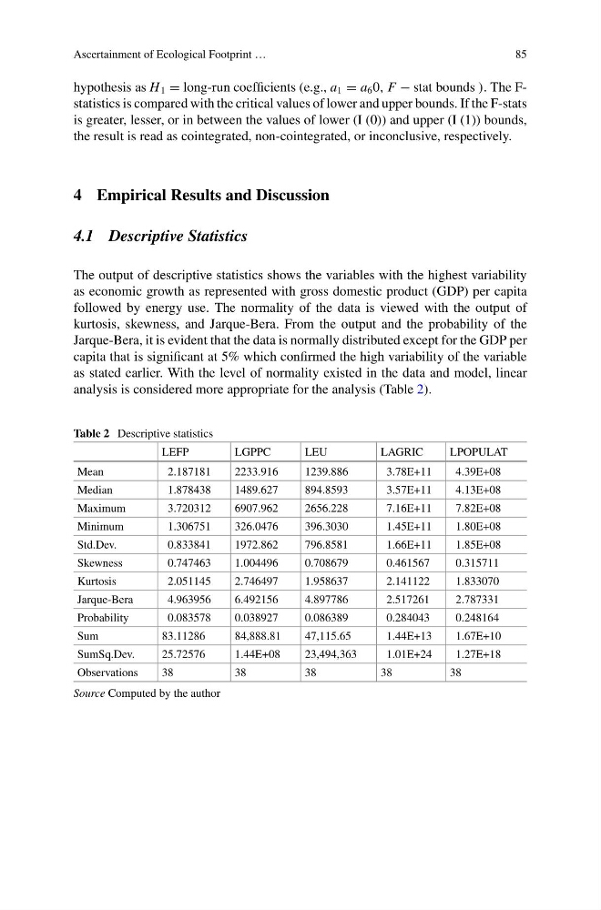
The output of descriptive statistics shows the variables with the highest variability
as economic growth as represented with gross domestic product (GDP) per capita
followed by energy use. The normality of the data is viewed with the output of
kurtosis, skewness, and Jarque-Bera. From the output and the probability of the
Jarque-Bera, it is evident that the data is normally distributed except for the GDP per
capita that is significant at 5% which confirmed the high variability of the variable
as stated earlier. With the level of normality existed in the data and model, linear
analysis is considered more appropriate for the analysis (Table 2).
Table 2 Descriptive statistics
LEFP
LGPPC
LEU
LAGRIC
LPOPULAT
Mean
2.187181
2233.916
1239.886
3.78E+11
4.39E+08
Median
1.878438
1489.627
894.8593
3.57E+11
4.13E+08
Maximum
3.720312
6907.962
2656.228
7.16E+11
7.82E+08
Minimum
1.306751
326.0476
396.3030
1.45E+11
1.80E+08
Std.Dev.
0.833841
1972.862
796.8581
1.66E+11
1.85E+08
Skewness
0.747463
1.004496
0.708679
0.461567
0.315711
Kurtosis
2.051145
2.746497
1.958637
2.141122
1.833070
Jarque-Bera
4.963956
6.492156
4.897786
2.517261
2.787331
Probability
0.083578
0.038927
0.086389
0.284043
0.248164
Sum
83.11286
84,888.81
47,115.65
1.44E+13
1.67E+10
SumSq.Dev.
25.72576
1.44E+08
23,494,363
1.01E+24
1.27E+18
Observations
38
38
38
38
38
Source Computed by the author
85
hypothesis as H 1 = long-run coefficients (e.g., a 1 = a 6 0, F − stat bounds ). The Fstatistics is compared with the critical values of lower and upper bounds. If the F-stats
is greater, lesser, or in between the values of lower (I (0)) and upper (I (1)) bounds,
the result is read as cointegrated, non-cointegrated, or inconclusive, respectively.
4 Empirical Results and Discussion
4.1 Descriptive Statistics
The output of descriptive statistics shows the variables with the highest variability
as economic growth as represented with gross domestic product (GDP) per capita
followed by energy use. The normality of the data is viewed with the output of
kurtosis, skewness, and Jarque-Bera. From the output and the probability of the
Jarque-Bera, it is evident that the data is normally distributed except for the GDP per
capita that is significant at 5% which confirmed the high variability of the variable
as stated earlier. With the level of normality existed in the data and model, linear
analysis is considered more appropriate for the analysis (Table 2).
Table 2 Descriptive statistics
LEFP
LGPPC
LEU
LAGRIC
LPOPULAT
Mean
2.187181
2233.916
1239.886
3.78E+11
4.39E+08
Median
1.878438
1489.627
894.8593
3.57E+11
4.13E+08
Maximum
3.720312
6907.962
2656.228
7.16E+11
7.82E+08
Minimum
1.306751
326.0476
396.3030
1.45E+11
1.80E+08
Std.Dev.
0.833841
1972.862
796.8581
1.66E+11
1.85E+08
Skewness
0.747463
1.004496
0.708679
0.461567
0.315711
Kurtosis
2.051145
2.746497
1.958637
2.141122
1.833070
Jarque-Bera
4.963956
6.492156
4.897786
2.517261
2.787331
Probability
0.083578
0.038927
0.086389
0.284043
0.248164
Sum
83.11286
84,888.81
47,115.65
1.44E+13
1.67E+10
SumSq.Dev.
25.72576
1.44E+08
23,494,363
1.01E+24
1.27E+18
Observations
38
38
38
38
38
Source Computed by the author