

2 Application of a Machine Learning Technique for Developing Short-Term Flood …
19
2.3.5 Runoff Forecasting Model Assessment and Feature
Reduction
It is commonly agreed that a direct comparison between model outputs and observations through goodness-of-fit statistics is not sufficient for correctly evaluating model
performance. When goodness-of-fit statistics are used alone, model assessment is
restricted to the mean model performance without taking into account the unbalanced
influence of outliers and extreme high (floods) or low (droughts) values. Therefore, to
complement model evaluation, we used graphical interpretation techniques to further
identify model weaknesses and applicability.
2.3.6 Goodness-Of-Fit Statistics
Among the variety of performance metrics, model residual mean (M E) measures the
average systematic difference between simulated and observed values. Whereas, the
average random differences can be measured by the mean squared error (M SE) and
the model residual variance (S
2
E Q ). For a enough number of observations, M SE =
M E
2
+ S
2
E Q . Therefore, the M SE comprises both a systematic (bias in the model)
and a random component (after bias correction) (Willems 2009). The systematic
error, which is the objective function, can be minimized through calibration. On the
contrary, the random component cannot be reduced since it is related to the inherent
stochastic nature of the inputs.
Nevertheless, the major disadvantage of the M E, M SE and S
2
E Q is their high
dependence on the magnitude of the variable of interest (e.g., runoff). Thus, we
selected the Nash–Sutcliffe efficiency (N SE) coefficient to measure the overall
model accuracy. The N SE coefficient is less sensitive to high extreme values when
compared to the previously mentioned performance metrics. In fact the N SE coefficient is an scaled version of the M SE; the N SE coefficient is the fraction of
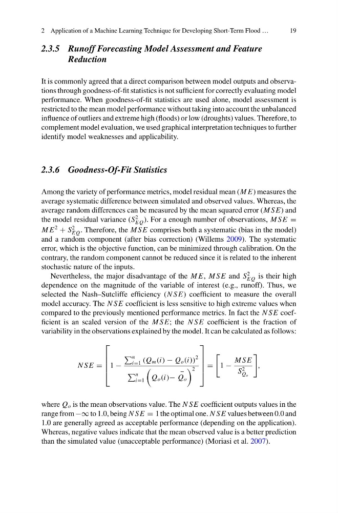
variability in the observations explained by the model. It can be calculated as follows:
N SE =
⎡
⎢
⎢
⎢
⎣
1 −
n
i=1 (Q m (i) − Q o (i))
2
n
i=1
Q o (i)−
−
Q o
2
⎤
⎥
⎥
⎥
⎦
=
1 −
M SE
S
2
Q o
,
where Q o is the mean observations value. The N SE coefficient outputs values in the
range from −∞ to 1.0, being N SE = 1 the optimal one. N SE values between 0.0 and
1.0 are generally agreed as acceptable performance (depending on the application).
Whereas, negative values indicate that the mean observed value is a better prediction
than the simulated value (unacceptable performance) (Moriasi et al. 2007).
19
2.3.5 Runoff Forecasting Model Assessment and Feature
Reduction
It is commonly agreed that a direct comparison between model outputs and observations through goodness-of-fit statistics is not sufficient for correctly evaluating model
performance. When goodness-of-fit statistics are used alone, model assessment is
restricted to the mean model performance without taking into account the unbalanced
influence of outliers and extreme high (floods) or low (droughts) values. Therefore, to
complement model evaluation, we used graphical interpretation techniques to further
identify model weaknesses and applicability.
2.3.6 Goodness-Of-Fit Statistics
Among the variety of performance metrics, model residual mean (M E) measures the
average systematic difference between simulated and observed values. Whereas, the
average random differences can be measured by the mean squared error (M SE) and
the model residual variance (S
2
E Q ). For a enough number of observations, M SE =
M E
2
+ S
2
E Q . Therefore, the M SE comprises both a systematic (bias in the model)
and a random component (after bias correction) (Willems 2009). The systematic
error, which is the objective function, can be minimized through calibration. On the
contrary, the random component cannot be reduced since it is related to the inherent
stochastic nature of the inputs.
Nevertheless, the major disadvantage of the M E, M SE and S
2
E Q is their high
dependence on the magnitude of the variable of interest (e.g., runoff). Thus, we
selected the Nash–Sutcliffe efficiency (N SE) coefficient to measure the overall
model accuracy. The N SE coefficient is less sensitive to high extreme values when
compared to the previously mentioned performance metrics. In fact the N SE coefficient is an scaled version of the M SE; the N SE coefficient is the fraction of
variability in the observations explained by the model. It can be calculated as follows:
N SE =
⎡
⎢
⎢
⎢
⎣
1 −
n
i=1 (Q m (i) − Q o (i))
2
n
i=1
Q o (i)−
−
Q o
2
⎤
⎥
⎥
⎥
⎦
=
1 −
M SE
S
2
Q o
,
where Q o is the mean observations value. The N SE coefficient outputs values in the
range from −∞ to 1.0, being N SE = 1 the optimal one. N SE values between 0.0 and
1.0 are generally agreed as acceptable performance (depending on the application).
Whereas, negative values indicate that the mean observed value is a better prediction
than the simulated value (unacceptable performance) (Moriasi et al. 2007).