

18
P. Muñoz et al.
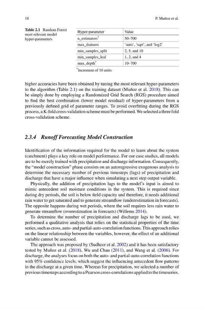
Table 2.1 Random Forest
most relevant model
hyper-parameters
Hyper-parameter
Value
n_estimators *
50–700
max_features
‘auto’, ‘sqrt’, and ‘log2’
min_samples_split
2, 5, and 10
min_samples_leaf
1, 2, and 4
max_depth *
10–700
* Increment of 10 units
higher accuracies have been obtained by tuning the most relevant hyper-parameters
to the algorithm (Table 2.1) on the training dataset (Muñoz et al. 2018). This can
be simply done by employing a Randomized Grid Search (RGS) procedure aimed
to find the best combination (lower model residual) of hyper-parameters from a
previously defined grid of parameter ranges. To avoid overfitting during the RGS
process, a K-fold cross-validation scheme must be performed. We selected a three fold
cross-validation scheme.
2.3.4 Runoff Forecasting Model Construction
Identification of the information required for the model to learn about the system
(catchment) plays a key role on model performance. For our case studies, all models
are to be merely trained with precipitation and discharge information. Consequently,
the “model construction” phase consists on an autoregressive exogenous analysis to
determine the necessary number of previous timesteps (lags) of precipitation and
discharge that have a major influence when simulating a next step output variable.
Physically, the addition of precipitation lags to the model’s input is aimed to
mimic antecedent soil moisture conditions in the system. This is required since
during dry periods, the soil is below field capacity and therefore, it needs additional
rain water to get saturated and to generate streamflow (underestimation in forecasts).
The opposite happens during wet periods, where the soil requires less rain water to
generate streamflow (overestimation in forecasts) (Willems 2014).
To determine the number of precipitation and discharge lags to be used, we
performed a qualitative analysis that relies on the statistical properties of the time
series, such as cross, auto- and partial-auto-correlation functions. This approach relies
on the linear relationship between the variables, however, the effect of an additional
variable cannot be assessed.
The approach was proposed by (Sudheer et al. 2002) and it has been satisfactory
tested by Muñoz et al. (2018), Wu and Chau (2011), and Wang et al. (2006). For
discharge, the analyses focus on both the auto- and partial-auto-correlation functions
with 95% confidence levels, which suggest the influencing antecedent flow patterns
in the discharge at a given time. Whereas for precipitation, we selected a number of
previous timesteps according to a Pearson cross-correlations applied to the timeseries.
P. Muñoz et al.
Table 2.1 Random Forest
most relevant model
hyper-parameters
Hyper-parameter
Value
n_estimators *
50–700
max_features
‘auto’, ‘sqrt’, and ‘log2’
min_samples_split
2, 5, and 10
min_samples_leaf
1, 2, and 4
max_depth *
10–700
* Increment of 10 units
higher accuracies have been obtained by tuning the most relevant hyper-parameters
to the algorithm (Table 2.1) on the training dataset (Muñoz et al. 2018). This can
be simply done by employing a Randomized Grid Search (RGS) procedure aimed
to find the best combination (lower model residual) of hyper-parameters from a
previously defined grid of parameter ranges. To avoid overfitting during the RGS
process, a K-fold cross-validation scheme must be performed. We selected a three fold
cross-validation scheme.
2.3.4 Runoff Forecasting Model Construction
Identification of the information required for the model to learn about the system
(catchment) plays a key role on model performance. For our case studies, all models
are to be merely trained with precipitation and discharge information. Consequently,
the “model construction” phase consists on an autoregressive exogenous analysis to
determine the necessary number of previous timesteps (lags) of precipitation and
discharge that have a major influence when simulating a next step output variable.
Physically, the addition of precipitation lags to the model’s input is aimed to
mimic antecedent soil moisture conditions in the system. This is required since
during dry periods, the soil is below field capacity and therefore, it needs additional
rain water to get saturated and to generate streamflow (underestimation in forecasts).
The opposite happens during wet periods, where the soil requires less rain water to
generate streamflow (overestimation in forecasts) (Willems 2014).
To determine the number of precipitation and discharge lags to be used, we
performed a qualitative analysis that relies on the statistical properties of the time
series, such as cross, auto- and partial-auto-correlation functions. This approach relies
on the linear relationship between the variables, however, the effect of an additional
variable cannot be assessed.
The approach was proposed by (Sudheer et al. 2002) and it has been satisfactory
tested by Muñoz et al. (2018), Wu and Chau (2011), and Wang et al. (2006). For
discharge, the analyses focus on both the auto- and partial-auto-correlation functions
with 95% confidence levels, which suggest the influencing antecedent flow patterns
in the discharge at a given time. Whereas for precipitation, we selected a number of
previous timesteps according to a Pearson cross-correlations applied to the timeseries.