

100
M. D. Setiawati et al.
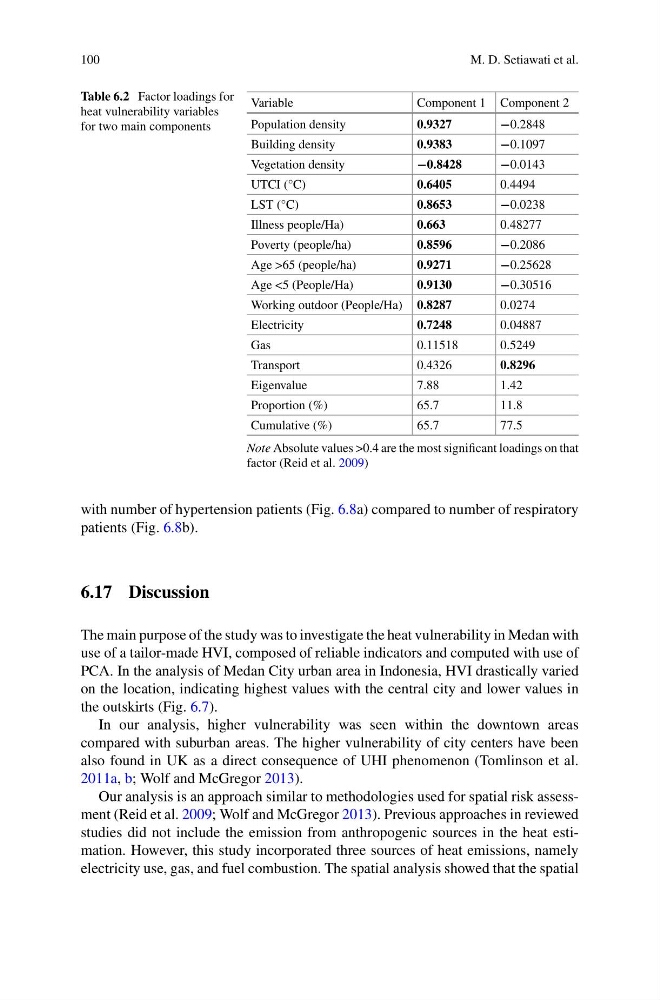
Table 6.2 Factor loadings for
heat vulnerability variables
for two main components
Variable
Component 1 Component 2
Population density
0.9327
−0.2848
Building density
0.9383
−0.1097
Vegetation density
−0.8428
−0.0143
UTCI (°C)
0.6405
0.4494
LST (°C)
0.8653
−0.0238
Illness people/Ha)
0.663
0.48277
Poverty (people/ha)
0.8596
−0.2086
Age >65 (people/ha)
0.9271
−0.25628
Age <5 (People/Ha)
0.9130
−0.30516
Working outdoor (People/Ha) 0.8287
0.0274
Electricity
0.7248
0.04887
Gas
0.11518
0.5249
Transport
0.4326
0.8296
Eigenvalue
7.88
1.42
Proportion (%)
65.7
11.8
Cumulative (%)
65.7
77.5
Note Absolute values >0.4 are the most significant loadings on that
factor (Reid et al. 2009)
with number of hypertension patients (Fig. 6.8a) compared to number of respiratory
patients (Fig. 6.8b).
6.17 Discussion
The main purpose of the study was to investigate the heat vulnerability in Medan with
use of a tailor-made HVI, composed of reliable indicators and computed with use of
PCA. In the analysis of Medan City urban area in Indonesia, HVI drastically varied
on the location, indicating highest values with the central city and lower values in
the outskirts (Fig. 6.7).
In our analysis, higher vulnerability was seen within the downtown areas
compared with suburban areas. The higher vulnerability of city centers have been
also found in UK as a direct consequence of UHI phenomenon (Tomlinson et al.
2011a, b; Wolf and McGregor 2013).
Our analysis is an approach similar to methodologies used for spatial risk assessment (Reid et al. 2009; Wolf and McGregor 2013). Previous approaches in reviewed
studies did not include the emission from anthropogenic sources in the heat estimation. However, this study incorporated three sources of heat emissions, namely
electricity use, gas, and fuel combustion. The spatial analysis showed that the spatial
M. D. Setiawati et al.
Table 6.2 Factor loadings for
heat vulnerability variables
for two main components
Variable
Component 1 Component 2
Population density
0.9327
−0.2848
Building density
0.9383
−0.1097
Vegetation density
−0.8428
−0.0143
UTCI (°C)
0.6405
0.4494
LST (°C)
0.8653
−0.0238
Illness people/Ha)
0.663
0.48277
Poverty (people/ha)
0.8596
−0.2086
Age >65 (people/ha)
0.9271
−0.25628
Age <5 (People/Ha)
0.9130
−0.30516
Working outdoor (People/Ha) 0.8287
0.0274
Electricity
0.7248
0.04887
Gas
0.11518
0.5249
Transport
0.4326
0.8296
Eigenvalue
7.88
1.42
Proportion (%)
65.7
11.8
Cumulative (%)
65.7
77.5
Note Absolute values >0.4 are the most significant loadings on that
factor (Reid et al. 2009)
with number of hypertension patients (Fig. 6.8a) compared to number of respiratory
patients (Fig. 6.8b).
6.17 Discussion
The main purpose of the study was to investigate the heat vulnerability in Medan with
use of a tailor-made HVI, composed of reliable indicators and computed with use of
PCA. In the analysis of Medan City urban area in Indonesia, HVI drastically varied
on the location, indicating highest values with the central city and lower values in
the outskirts (Fig. 6.7).
In our analysis, higher vulnerability was seen within the downtown areas
compared with suburban areas. The higher vulnerability of city centers have been
also found in UK as a direct consequence of UHI phenomenon (Tomlinson et al.
2011a, b; Wolf and McGregor 2013).
Our analysis is an approach similar to methodologies used for spatial risk assessment (Reid et al. 2009; Wolf and McGregor 2013). Previous approaches in reviewed
studies did not include the emission from anthropogenic sources in the heat estimation. However, this study incorporated three sources of heat emissions, namely
electricity use, gas, and fuel combustion. The spatial analysis showed that the spatial