

assumption (consumption divided by income) made by Wackernagel 1998), that also
found income to be associated with larger Footprints. Lenzen and Murray (2001)
addressed this in some detail, suggesting that demographic factors (including
income, expenditure, size, and the location of households) be examined since for
an income increase of 10%, they found the Ecological Footprint to increase 3.8%.
Moreover, they posited high-income consumption to be less ‘land disturbing’ than at
10
9
8
7
6
5
4
3
Footprint
2
1
0
0
2000
4000
Income (USD)
6000
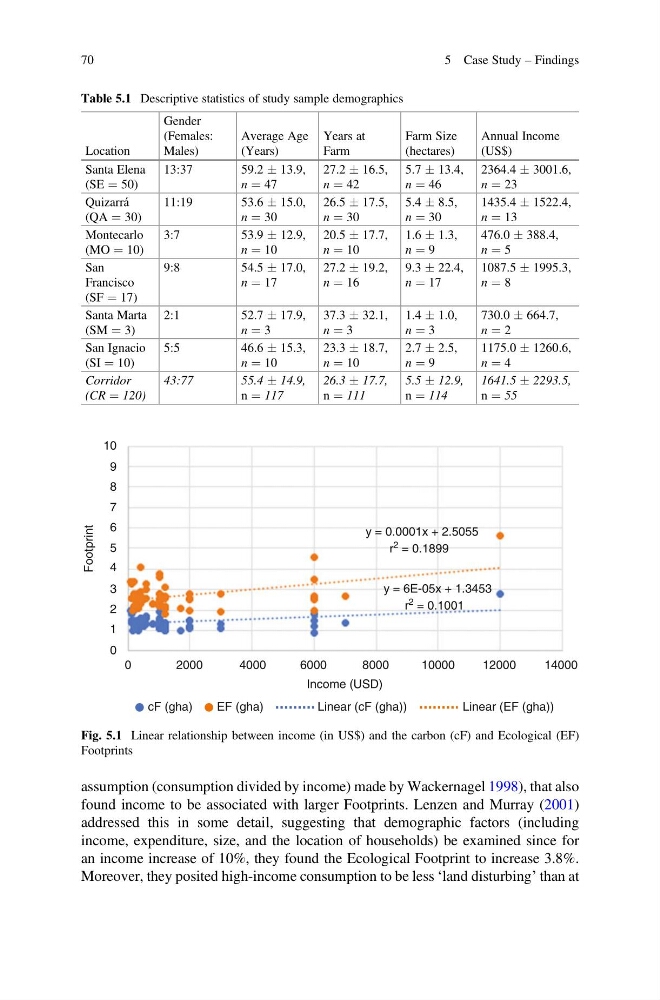
y = 0.0001x + 2.5055
r
2 = 0.1899
y = 6E-05x + 1.3453
r
2 = 0.1001
8000
10000
12000
14000
cF (gha)
EF (gha)
Linear (cF (gha))
Linear (EF (gha))
Fig. 5.1 Linear relationship between income (in US$) and the carbon (cF) and Ecological (EF)
Footprints
Table 5.1 Descriptive statistics of study sample demographics
Location
Gender
(Females:
Males)
Average Age
(Years)
Years at
Farm
Farm Size
(hectares)
Annual Income
(US$)
Santa Elena
(SE ¼ 50)
13:37
59.2 Æ 13.9,
n ¼ 47
27.2 Æ 16.5,
n ¼ 42
5.7 Æ 13.4,
n ¼ 46
2364.4 Æ 3001.6,
n ¼ 23
Quizarrá
(QA ¼ 30)
11:19
53.6 Æ 15.0,
n ¼ 30
26.5 Æ 17.5,
n ¼ 30
5.4 Æ 8.5,
n ¼ 30
1435.4 Æ 1522.4,
n ¼ 13
Montecarlo
(MO ¼ 10)
3:7
53.9 Æ 12.9,
n ¼ 10
20.5 Æ 17.7,
n ¼ 10
1.6 Æ 1.3,
n ¼ 9
476.0 Æ 388.4,
n ¼ 5
San
Francisco
(SF ¼ 17)
9:8
54.5 Æ 17.0,
n ¼ 17
27.2 Æ 19.2,
n ¼ 16
9.3 Æ 22.4,
n ¼ 17
1087.5 Æ 1995.3,
n ¼ 8
Santa Marta
(SM ¼ 3)
2:1
52.7 Æ 17.9,
n ¼ 3
37.3 Æ 32.1,
n ¼ 3
1.4 Æ 1.0,
n ¼ 3
730.0 Æ 664.7,
n ¼ 2
San Ignacio
(SI ¼ 10)
5:5
46.6 Æ 15.3,
n ¼ 10
23.3 Æ 18.7,
n ¼ 10
2.7 Æ 2.5,
n ¼ 9
1175.0 Æ 1260.6,
n ¼ 4
Corridor
(CR ¼ 120)
43:77
55.4 Æ 14.9,
n ¼ 117
26.3 Æ 17.7,
n ¼ 111
5.5 Æ 12.9,
n ¼ 114
1641.5 Æ 2293.5,
n ¼ 55
70
5 Case Study – Findings
found income to be associated with larger Footprints. Lenzen and Murray (2001)
addressed this in some detail, suggesting that demographic factors (including
income, expenditure, size, and the location of households) be examined since for
an income increase of 10%, they found the Ecological Footprint to increase 3.8%.
Moreover, they posited high-income consumption to be less ‘land disturbing’ than at
10
9
8
7
6
5
4
3
Footprint
2
1
0
0
2000
4000
Income (USD)
6000
y = 0.0001x + 2.5055
r
2 = 0.1899
y = 6E-05x + 1.3453
r
2 = 0.1001
8000
10000
12000
14000
cF (gha)
EF (gha)
Linear (cF (gha))
Linear (EF (gha))
Fig. 5.1 Linear relationship between income (in US$) and the carbon (cF) and Ecological (EF)
Footprints
Table 5.1 Descriptive statistics of study sample demographics
Location
Gender
(Females:
Males)
Average Age
(Years)
Years at
Farm
Farm Size
(hectares)
Annual Income
(US$)
Santa Elena
(SE ¼ 50)
13:37
59.2 Æ 13.9,
n ¼ 47
27.2 Æ 16.5,
n ¼ 42
5.7 Æ 13.4,
n ¼ 46
2364.4 Æ 3001.6,
n ¼ 23
Quizarrá
(QA ¼ 30)
11:19
53.6 Æ 15.0,
n ¼ 30
26.5 Æ 17.5,
n ¼ 30
5.4 Æ 8.5,
n ¼ 30
1435.4 Æ 1522.4,
n ¼ 13
Montecarlo
(MO ¼ 10)
3:7
53.9 Æ 12.9,
n ¼ 10
20.5 Æ 17.7,
n ¼ 10
1.6 Æ 1.3,
n ¼ 9
476.0 Æ 388.4,
n ¼ 5
San
Francisco
(SF ¼ 17)
9:8
54.5 Æ 17.0,
n ¼ 17
27.2 Æ 19.2,
n ¼ 16
9.3 Æ 22.4,
n ¼ 17
1087.5 Æ 1995.3,
n ¼ 8
Santa Marta
(SM ¼ 3)
2:1
52.7 Æ 17.9,
n ¼ 3
37.3 Æ 32.1,
n ¼ 3
1.4 Æ 1.0,
n ¼ 3
730.0 Æ 664.7,
n ¼ 2
San Ignacio
(SI ¼ 10)
5:5
46.6 Æ 15.3,
n ¼ 10
23.3 Æ 18.7,
n ¼ 10
2.7 Æ 2.5,
n ¼ 9
1175.0 Æ 1260.6,
n ¼ 4
Corridor
(CR ¼ 120)
43:77
55.4 Æ 14.9,
n ¼ 117
26.3 Æ 17.7,
n ¼ 111
5.5 Æ 12.9,
n ¼ 114
1641.5 Æ 2293.5,
n ¼ 55
70
5 Case Study – Findings