

How Econometrics Can Help Us Understand the Effects …
29
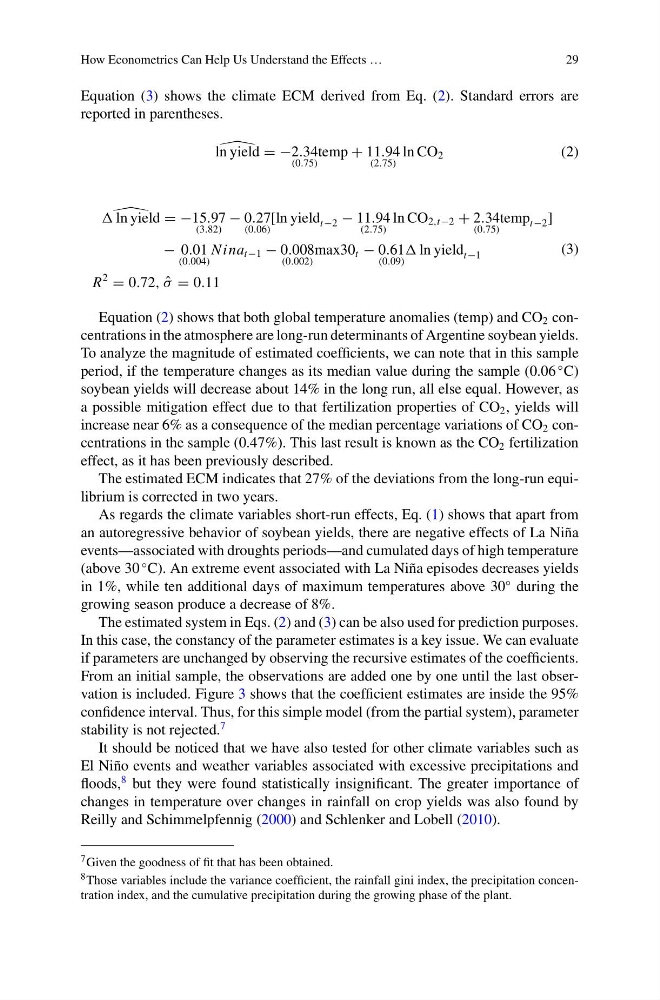
Equation (3) shows the climate ECM derived from Eq. (2). Standard errors are
reported in parentheses.
ln yield = −2.34
(0.75)
temp + 11.94
(2.75)
ln CO 2
(2)
ln yield = −15.97
(3.82)
− 0.27
(0.06)
[ln yield t−2 − 11.94
(2.75)
ln CO 2,t−2 + 2.34
(0.75)
temp t−2 ]
− 0.01
(0.004)
Nina t−1 − 0.008
(0.002)
max30 t − 0.61
(0.09)
ln yield t−1
R
2
= 0.72, ˆ
σ = 0.11
(3)
Equation (2) shows that both global temperature anomalies (temp) and CO 2 concentrations in the atmosphere are long-run determinants of Argentine soybean yields.
To analyze the magnitude of estimated coefficients, we can note that in this sample
period, if the temperature changes as its median value during the sample (0.06
◦ C)
soybean yields will decrease about 14% in the long run, all else equal. However, as
a possible mitigation effect due to that fertilization properties of CO 2 , yields will
increase near 6% as a consequence of the median percentage variations of CO 2 concentrations in the sample (0.47%). This last result is known as the CO 2 fertilization
effect, as it has been previously described.
The estimated ECM indicates that 27% of the deviations from the long-run equilibrium is corrected in two years.
As regards the climate variables short-run effects, Eq. (1) shows that apart from
an autoregressive behavior of soybean yields, there are negative effects of La Niña
events—associated with droughts periods—and cumulated days of high temperature
(above 30
◦ C). An extreme event associated with La Niña episodes decreases yields
in 1%, while ten additional days of maximum temperatures above 30
◦ during the
growing season produce a decrease of 8%.
The estimated system in Eqs. (2) and (3) can be also used for prediction purposes.
In this case, the constancy of the parameter estimates is a key issue. We can evaluate
if parameters are unchanged by observing the recursive estimates of the coefficients.
From an initial sample, the observations are added one by one until the last observation is included. Figure 3 shows that the coefficient estimates are inside the 95%
confidence interval. Thus, for this simple model (from the partial system), parameter
stability is not rejected.
7
It should be noticed that we have also tested for other climate variables such as
El Niño events and weather variables associated with excessive precipitations and
floods,
8 but they were found statistically insignificant. The greater importance of
changes in temperature over changes in rainfall on crop yields was also found by
Reilly and Schimmelpfennig (2000) and Schlenker and Lobell (2010).
7 Given the goodness of fit that has been obtained.
8 Those variables include the variance coefficient, the rainfall gini index, the precipitation concentration index, and the cumulative precipitation during the growing phase of the plant.
29
Equation (3) shows the climate ECM derived from Eq. (2). Standard errors are
reported in parentheses.
ln yield = −2.34
(0.75)
temp + 11.94
(2.75)
ln CO 2
(2)
ln yield = −15.97
(3.82)
− 0.27
(0.06)
[ln yield t−2 − 11.94
(2.75)
ln CO 2,t−2 + 2.34
(0.75)
temp t−2 ]
− 0.01
(0.004)
Nina t−1 − 0.008
(0.002)
max30 t − 0.61
(0.09)
ln yield t−1
R
2
= 0.72, ˆ
σ = 0.11
(3)
Equation (2) shows that both global temperature anomalies (temp) and CO 2 concentrations in the atmosphere are long-run determinants of Argentine soybean yields.
To analyze the magnitude of estimated coefficients, we can note that in this sample
period, if the temperature changes as its median value during the sample (0.06
◦ C)
soybean yields will decrease about 14% in the long run, all else equal. However, as
a possible mitigation effect due to that fertilization properties of CO 2 , yields will
increase near 6% as a consequence of the median percentage variations of CO 2 concentrations in the sample (0.47%). This last result is known as the CO 2 fertilization
effect, as it has been previously described.
The estimated ECM indicates that 27% of the deviations from the long-run equilibrium is corrected in two years.
As regards the climate variables short-run effects, Eq. (1) shows that apart from
an autoregressive behavior of soybean yields, there are negative effects of La Niña
events—associated with droughts periods—and cumulated days of high temperature
(above 30
◦ C). An extreme event associated with La Niña episodes decreases yields
in 1%, while ten additional days of maximum temperatures above 30
◦ during the
growing season produce a decrease of 8%.
The estimated system in Eqs. (2) and (3) can be also used for prediction purposes.
In this case, the constancy of the parameter estimates is a key issue. We can evaluate
if parameters are unchanged by observing the recursive estimates of the coefficients.
From an initial sample, the observations are added one by one until the last observation is included. Figure 3 shows that the coefficient estimates are inside the 95%
confidence interval. Thus, for this simple model (from the partial system), parameter
stability is not rejected.
7
It should be noticed that we have also tested for other climate variables such as
El Niño events and weather variables associated with excessive precipitations and
floods,
8 but they were found statistically insignificant. The greater importance of
changes in temperature over changes in rainfall on crop yields was also found by
Reilly and Schimmelpfennig (2000) and Schlenker and Lobell (2010).
7 Given the goodness of fit that has been obtained.
8 Those variables include the variance coefficient, the rainfall gini index, the precipitation concentration index, and the cumulative precipitation during the growing phase of the plant.