

How Econometrics Can Help Us Understand the Effects …
23
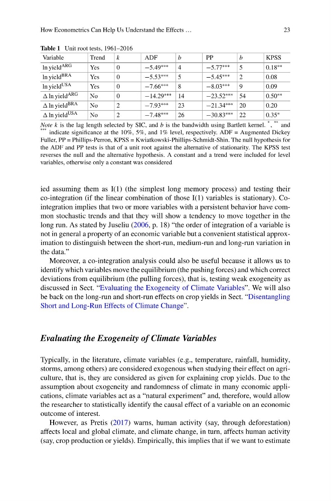
Table 1 Unit root tests, 1961–2016
Variable
Trend
k
ADF
b
PP
b
KPSS
ln yield ARG
Yes
0
−5.49 ∗∗∗
4
−5.77 ∗∗∗
5
0.18 ∗∗
ln yield BRA
Yes
0
−5.53 ∗∗∗
5
−5.45 ∗∗∗
2
0.08
ln yield USA
Yes
0
−7.66 ∗∗∗
8
−8.03 ∗∗∗
9
0.09
ln yield ARG
No
0
−14.29 ∗∗∗ 14
−23.52 ∗∗∗ 54
0.50 ∗∗
ln yield BRA
No
2
−7.93 ∗∗∗
23
−21.34 ∗∗∗ 20
0.20
ln yield USA
No
2
−7.48 ∗∗∗
26
−30.83 ∗∗∗ 22
0.35 ∗
Note k is the lag length selected by SIC, and b is the bandwidth using Bartlett kernel.
∗ ,
∗∗ and
∗∗∗ indicate significance at the 10%, 5%, and 1% level, respectively. ADF = Augmented Dickey
Fuller, PP = Phillips-Perron, KPSS = Kwiatkowski-Phillips-Schmidt-Shin. The null hypothesis for
the ADF and PP tests is that of a unit root against the alternative of stationarity. The KPSS test
reverses the null and the alternative hypothesis. A constant and a trend were included for level
variables, otherwise only a constant was considered
ied assuming them as I(1) (the simplest long memory process) and testing their
co-integration (if the linear combination of those I(1) variables is stationary). Cointegration implies that two or more variables with a persistent behavior have common stochastic trends and that they will show a tendency to move together in the
long run. As stated by Juseliu (2006, p. 18) “the order of integration of a variable is
not in general a property of an economic variable but a convenient statistical approximation to distinguish between the short-run, medium-run and long-run variation in
the data.”
Moreover, a co-integration analysis could also be useful because it allows us to
identify which variables move the equilibrium (the pushing forces) and which correct
deviations from equilibrium (the pulling forces), that is, testing weak exogeneity as
discussed in Sect. “Evaluating the Exogeneity of Climate Variables”. We will also
be back on the long-run and short-run effects on crop yields in Sect. “Disentangling
Short and Long-Run Effects of Climate Change”.
Evaluating the Exogeneity of Climate Variables
Typically, in the literature, climate variables (e.g., temperature, rainfall, humidity,
storms, among others) are considered exogenous when studying their effect on agriculture, that is, they are considered as given for explaining crop yields. Due to the
assumption about exogeneity and randomness of climate in many economic applications, climate variables act as a “natural experiment” and, therefore, would allow
the researcher to statistically identify the causal effect of a variable on an economic
outcome of interest.
However, as Pretis (2017) warns, human activity (say, through deforestation)
affects local and global climate, and climate change, in turn, affects human activity
(say, crop production or yields). Empirically, this implies that if we want to estimate
23
Table 1 Unit root tests, 1961–2016
Variable
Trend
k
ADF
b
PP
b
KPSS
ln yield ARG
Yes
0
−5.49 ∗∗∗
4
−5.77 ∗∗∗
5
0.18 ∗∗
ln yield BRA
Yes
0
−5.53 ∗∗∗
5
−5.45 ∗∗∗
2
0.08
ln yield USA
Yes
0
−7.66 ∗∗∗
8
−8.03 ∗∗∗
9
0.09
ln yield ARG
No
0
−14.29 ∗∗∗ 14
−23.52 ∗∗∗ 54
0.50 ∗∗
ln yield BRA
No
2
−7.93 ∗∗∗
23
−21.34 ∗∗∗ 20
0.20
ln yield USA
No
2
−7.48 ∗∗∗
26
−30.83 ∗∗∗ 22
0.35 ∗
Note k is the lag length selected by SIC, and b is the bandwidth using Bartlett kernel.
∗ ,
∗∗ and
∗∗∗ indicate significance at the 10%, 5%, and 1% level, respectively. ADF = Augmented Dickey
Fuller, PP = Phillips-Perron, KPSS = Kwiatkowski-Phillips-Schmidt-Shin. The null hypothesis for
the ADF and PP tests is that of a unit root against the alternative of stationarity. The KPSS test
reverses the null and the alternative hypothesis. A constant and a trend were included for level
variables, otherwise only a constant was considered
ied assuming them as I(1) (the simplest long memory process) and testing their
co-integration (if the linear combination of those I(1) variables is stationary). Cointegration implies that two or more variables with a persistent behavior have common stochastic trends and that they will show a tendency to move together in the
long run. As stated by Juseliu (2006, p. 18) “the order of integration of a variable is
not in general a property of an economic variable but a convenient statistical approximation to distinguish between the short-run, medium-run and long-run variation in
the data.”
Moreover, a co-integration analysis could also be useful because it allows us to
identify which variables move the equilibrium (the pushing forces) and which correct
deviations from equilibrium (the pulling forces), that is, testing weak exogeneity as
discussed in Sect. “Evaluating the Exogeneity of Climate Variables”. We will also
be back on the long-run and short-run effects on crop yields in Sect. “Disentangling
Short and Long-Run Effects of Climate Change”.
Evaluating the Exogeneity of Climate Variables
Typically, in the literature, climate variables (e.g., temperature, rainfall, humidity,
storms, among others) are considered exogenous when studying their effect on agriculture, that is, they are considered as given for explaining crop yields. Due to the
assumption about exogeneity and randomness of climate in many economic applications, climate variables act as a “natural experiment” and, therefore, would allow
the researcher to statistically identify the causal effect of a variable on an economic
outcome of interest.
However, as Pretis (2017) warns, human activity (say, through deforestation)
affects local and global climate, and climate change, in turn, affects human activity
(say, crop production or yields). Empirically, this implies that if we want to estimate