

• Cumulative Percentage of Variance and Eigenvalue >1 Rule: The eigenvalue explains the degree of
variation explained by a factor. The eigenvalue of 1
represents an extensive amount of variation (Field,
2009). There is no fixed threshold, although the
researchers have recommended certain percentages.
For instance, Hair et al. (2010) describe that in natural
sciences, the explained variance should be at least
95% and in the humanities, the explained variance can
be as low as 50–60%.
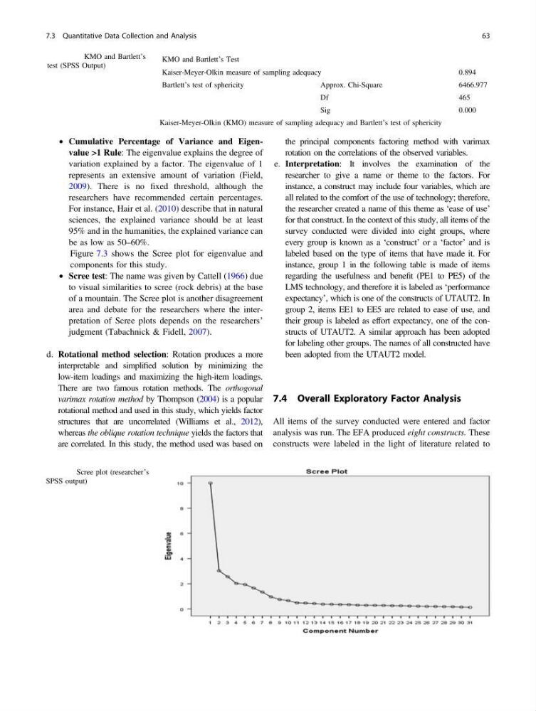
Figure 7.3 shows the Scree plot for eigenvalue and
components for this study.
• Scree test: The name was given by Cattell (1966) due
to visual similarities to scree (rock debris) at the base
of a mountain. The Scree plot is another disagreement
area and debate for the researchers where the interpretation of Scree plots depends on the researchers’
judgment (Tabachnick & Fidell, 2007).
d. Rotational method selection: Rotation produces a more
interpretable and simplified solution by minimizing the
low-item loadings and maximizing the high-item loadings.
There are two famous rotation methods. The orthogonal
varimax rotation method by Thompson (2004) is a popular
rotational method and used in this study, which yields factor
structures that are uncorrelated (Williams et al., 2012),
whereas the oblique rotation technique yields the factors that
are correlated. In this study, the method used was based on
the principal components factoring method with varimax
rotation on the correlations of the observed variables.
e. Interpretation: It involves the examination of the
researcher to give a name or theme to the factors. For
instance, a construct may include four variables, which are
all related to the comfort of the use of technology; therefore,
the researcher created a name of this theme as ‘ease of use’
for that construct. In the context of this study, all items of the
survey conducted were divided into eight groups, where
every group is known as a ‘construct’ or a ‘factor’ and is
labeled based on the type of items that have made it. For
instance, group 1 in the following table is made of items
regarding the usefulness and benefit (PE1 to PE5) of the
LMS technology, and therefore it is labeled as ‘performance
expectancy’, which is one of the constructs of UTAUT2. In
group 2, items EE1 to EE5 are related to ease of use, and
their group is labeled as effort expectancy, one of the constructs of UTAUT2. A similar approach has been adopted
for labeling other groups. The names of all constructed have
been adopted from the UTAUT2 model.
7.4 Overall Exploratory Factor Analysis
All items of the survey conducted were entered and factor
analysis was run. The EFA produced eight constructs. These
constructs were labeled in the light of literature related to
Table 7.2 KMO and Bartlett’s
test (SPSS Output)
KMO and Bartlett’s Test
Kaiser-Meyer-Olkin measure of sampling adequacy
0.894
Bartlett’s test of sphericity
Approx. Chi-Square
6466.977
Df
465
Sig
0.000
Kaiser-Meyer-Olkin (KMO) measure of sampling adequacy and Bartlett’s test of sphericity
Fig. 7.3 Scree plot (researcher’s
SPSS output)
7.3 Quantitative Data Collection and Analysis
63
variation explained by a factor. The eigenvalue of 1
represents an extensive amount of variation (Field,
2009). There is no fixed threshold, although the
researchers have recommended certain percentages.
For instance, Hair et al. (2010) describe that in natural
sciences, the explained variance should be at least
95% and in the humanities, the explained variance can
be as low as 50–60%.
Figure 7.3 shows the Scree plot for eigenvalue and
components for this study.
• Scree test: The name was given by Cattell (1966) due
to visual similarities to scree (rock debris) at the base
of a mountain. The Scree plot is another disagreement
area and debate for the researchers where the interpretation of Scree plots depends on the researchers’
judgment (Tabachnick & Fidell, 2007).
d. Rotational method selection: Rotation produces a more
interpretable and simplified solution by minimizing the
low-item loadings and maximizing the high-item loadings.
There are two famous rotation methods. The orthogonal
varimax rotation method by Thompson (2004) is a popular
rotational method and used in this study, which yields factor
structures that are uncorrelated (Williams et al., 2012),
whereas the oblique rotation technique yields the factors that
are correlated. In this study, the method used was based on
the principal components factoring method with varimax
rotation on the correlations of the observed variables.
e. Interpretation: It involves the examination of the
researcher to give a name or theme to the factors. For
instance, a construct may include four variables, which are
all related to the comfort of the use of technology; therefore,
the researcher created a name of this theme as ‘ease of use’
for that construct. In the context of this study, all items of the
survey conducted were divided into eight groups, where
every group is known as a ‘construct’ or a ‘factor’ and is
labeled based on the type of items that have made it. For
instance, group 1 in the following table is made of items
regarding the usefulness and benefit (PE1 to PE5) of the
LMS technology, and therefore it is labeled as ‘performance
expectancy’, which is one of the constructs of UTAUT2. In
group 2, items EE1 to EE5 are related to ease of use, and
their group is labeled as effort expectancy, one of the constructs of UTAUT2. A similar approach has been adopted
for labeling other groups. The names of all constructed have
been adopted from the UTAUT2 model.
7.4 Overall Exploratory Factor Analysis
All items of the survey conducted were entered and factor
analysis was run. The EFA produced eight constructs. These
constructs were labeled in the light of literature related to
Table 7.2 KMO and Bartlett’s
test (SPSS Output)
KMO and Bartlett’s Test
Kaiser-Meyer-Olkin measure of sampling adequacy
0.894
Bartlett’s test of sphericity
Approx. Chi-Square
6466.977
Df
465
Sig
0.000
Kaiser-Meyer-Olkin (KMO) measure of sampling adequacy and Bartlett’s test of sphericity
Fig. 7.3 Scree plot (researcher’s
SPSS output)
7.3 Quantitative Data Collection and Analysis
63