

98
L. Prabhu et al.
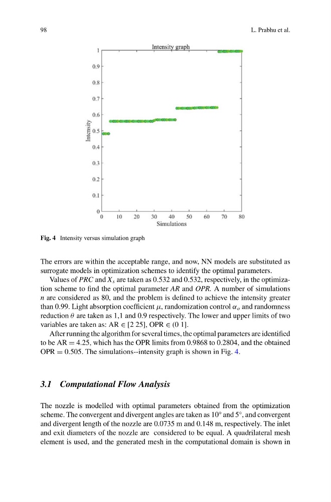
Fig. 4 Intensity versus simulation graph
The errors are within the acceptable range, and now, NN models are substituted as
surrogate models in optimization schemes to identify the optimal parameters.
Values of PRC and X s are taken as 0.532 and 0.532, respectively, in the optimization scheme to find the optimal parameter AR and OPR. A number of simulations
n are considered as 80, and the problem is defined to achieve the intensity greater
than 0.99. Light absorption coefficient μ, randomization control α o and randomness
reduction θ are taken as 1,1 and 0.9 respectively. The lower and upper limits of two
variables are taken as: AR ∈ [2 25], OPR ∈ (0 1].
After running the algorithm for several times, the optimal parameters are identified
to be AR = 4.25, which has the OPR limits from 0.9868 to 0.2804, and the obtained
OPR = 0.505. The simulations--intensity graph is shown in Fig. 4.
3.1 Computational Flow Analysis
The nozzle is modelled with optimal parameters obtained from the optimization
scheme. The convergent and divergent angles are taken as 10° and 5°, and convergent
and divergent length of the nozzle are 0.0735 m and 0.148 m, respectively. The inlet
and exit diameters of the nozzle are considered to be equal. A quadrilateral mesh
element is used, and the generated mesh in the computational domain is shown in
L. Prabhu et al.
Fig. 4 Intensity versus simulation graph
The errors are within the acceptable range, and now, NN models are substituted as
surrogate models in optimization schemes to identify the optimal parameters.
Values of PRC and X s are taken as 0.532 and 0.532, respectively, in the optimization scheme to find the optimal parameter AR and OPR. A number of simulations
n are considered as 80, and the problem is defined to achieve the intensity greater
than 0.99. Light absorption coefficient μ, randomization control α o and randomness
reduction θ are taken as 1,1 and 0.9 respectively. The lower and upper limits of two
variables are taken as: AR ∈ [2 25], OPR ∈ (0 1].
After running the algorithm for several times, the optimal parameters are identified
to be AR = 4.25, which has the OPR limits from 0.9868 to 0.2804, and the obtained
OPR = 0.505. The simulations--intensity graph is shown in Fig. 4.
3.1 Computational Flow Analysis
The nozzle is modelled with optimal parameters obtained from the optimization
scheme. The convergent and divergent angles are taken as 10° and 5°, and convergent
and divergent length of the nozzle are 0.0735 m and 0.148 m, respectively. The inlet
and exit diameters of the nozzle are considered to be equal. A quadrilateral mesh
element is used, and the generated mesh in the computational domain is shown in