

4.3 Numeral Examples
69
0
20
40
60
80
100
0.5
1
1.5
2
2.5
3
3.5
t/s
mode
mode
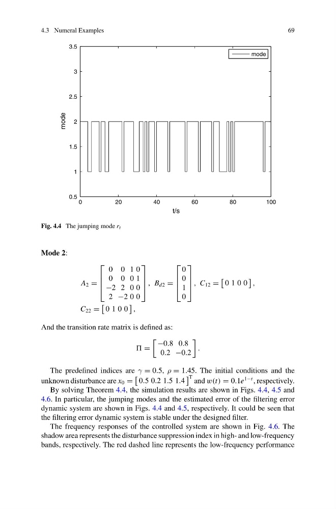
Fig. 4.4 The jumping mode r t
Mode 2:
A 2 =
⎡
⎢
⎢
⎣
0 0 1 0
0 0 0 1
−2 2 0 0
2 −2 0 0
⎤
⎥
⎥
⎦ , B d2 =
⎡
⎢
⎢
⎣
0
0
1
0
⎤
⎥
⎥
⎦ , C 12 =
0 1 0 0
,
C 22 =
0 1 0 0
,
And the transition rate matrix is defined as:
=
−0.8 0.8
0.2 −0.2
.
The predefined indices are γ = 0.5, ρ = 1.45. The initial conditions and the
unknown disturbance are x 0 =
0.5 0.2 1.5 1.4
T and w(t) = 0.1e
1−t , respectively.
By solving Theorem 4.4, the simulation results are shown in Figs. 4.4, 4.5 and
4.6. In particular, the jumping modes and the estimated error of the filtering error
dynamic system are shown in Figs. 4.4 and 4.5, respectively. It could be seen that
the filtering error dynamic system is stable under the designed filter.
The frequency responses of the controlled system are shown in Fig. 4.6. The
shadow area represents the disturbance suppression index in high- and low-frequency
bands, respectively. The red dashed line represents the low-frequency performance
69
0
20
40
60
80
100
0.5
1
1.5
2
2.5
3
3.5
t/s
mode
mode
Fig. 4.4 The jumping mode r t
Mode 2:
A 2 =
⎡
⎢
⎢
⎣
0 0 1 0
0 0 0 1
−2 2 0 0
2 −2 0 0
⎤
⎥
⎥
⎦ , B d2 =
⎡
⎢
⎢
⎣
0
0
1
0
⎤
⎥
⎥
⎦ , C 12 =
0 1 0 0
,
C 22 =
0 1 0 0
,
And the transition rate matrix is defined as:
=
−0.8 0.8
0.2 −0.2
.
The predefined indices are γ = 0.5, ρ = 1.45. The initial conditions and the
unknown disturbance are x 0 =
0.5 0.2 1.5 1.4
T and w(t) = 0.1e
1−t , respectively.
By solving Theorem 4.4, the simulation results are shown in Figs. 4.4, 4.5 and
4.6. In particular, the jumping modes and the estimated error of the filtering error
dynamic system are shown in Figs. 4.4 and 4.5, respectively. It could be seen that
the filtering error dynamic system is stable under the designed filter.
The frequency responses of the controlled system are shown in Fig. 4.6. The
shadow area represents the disturbance suppression index in high- and low-frequency
bands, respectively. The red dashed line represents the low-frequency performance