

56
4 Finite-Frequency Robust Filtering for Multi-model Jumping System
take a different value of matrix to describe the other finite frequency performance
of the considered system, such as =
0 −I
−I 0
for the positive realness.
4.1.2 Finite Frequency Performance Analysis and Filter
Design
Taking middle-frequency filtering for example, the finite frequency performance
analysis, filter design, and stability conditions are given in sequence.
A. Finite Frequency Performance Analysis
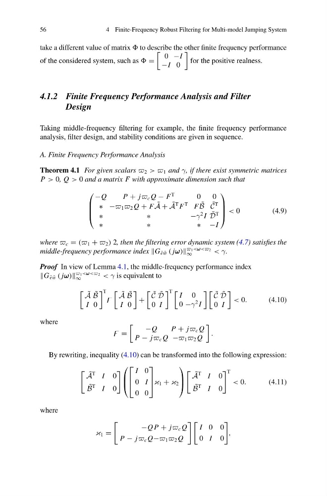
Theorem 4.1 For given scalars 2 > 1 and γ, if there exist symmetric matrices
P > 0, Q > 0 and a matrix F with approximate dimension such that
⎛
⎜
⎜
⎝
−Q
P+ j c Q − F
T
0
0
∗ − 1 2 Q + F ˜
A + ˜
A
T F
T F ˜
B ˜
C
T
∗
∗
− γ
2 I ˜
D
T
∗
∗
∗ − I
⎞
⎟
⎟
⎠ < 0
(4.9)
where c = ( 1 + 2 ) 2, then the filtering error dynamic system (4.7) satisfies the
middle-frequency performance index G ˜
e ˜
w ( jω ω ω)
1 <ω ω ω< 2
∞
< γ.
Proof In view of Lemma 4.1, the middle-frequency performance index
G ˜
e ˜
w ( jω ω ω)
1 <ω ω ω< 2
∞
< γ is equivalent to
˜
A ˜
B
I 0
T
˜
A ˜
B
I 0
+
˜
C ˜
D
0 I
T
I 0
0 −γ
2 I
˜
C ˜
D
0 I
< 0.
(4.10)
where
=
−Q
P + j c Q
P − j c Q − 1 2 Q
.
By rewriting, inequality (4.10) can be transformed into the following expression:
˜
A
T I 0
˜
B
T I 0
⎛
⎜
⎝
⎡
⎢
⎣
I 0
0 I
0 0
⎤
⎥
⎦κ1 + κ 2
⎞
⎟
⎠
˜
A
T I 0
˜
B
T I 0
T
< 0.
(4.11)
where
κ 1 =
−Q P + j c Q
P − j c Q− 1 2 Q
I 0 0
0 I 0
,
4 Finite-Frequency Robust Filtering for Multi-model Jumping System
take a different value of matrix to describe the other finite frequency performance
of the considered system, such as =
0 −I
−I 0
for the positive realness.
4.1.2 Finite Frequency Performance Analysis and Filter
Design
Taking middle-frequency filtering for example, the finite frequency performance
analysis, filter design, and stability conditions are given in sequence.
A. Finite Frequency Performance Analysis
Theorem 4.1 For given scalars 2 > 1 and γ, if there exist symmetric matrices
P > 0, Q > 0 and a matrix F with approximate dimension such that
⎛
⎜
⎜
⎝
−Q
P+ j c Q − F
T
0
0
∗ − 1 2 Q + F ˜
A + ˜
A
T F
T F ˜
B ˜
C
T
∗
∗
− γ
2 I ˜
D
T
∗
∗
∗ − I
⎞
⎟
⎟
⎠ < 0
(4.9)
where c = ( 1 + 2 ) 2, then the filtering error dynamic system (4.7) satisfies the
middle-frequency performance index G ˜
e ˜
w ( jω ω ω)
1 <ω ω ω< 2
∞
< γ.
Proof In view of Lemma 4.1, the middle-frequency performance index
G ˜
e ˜
w ( jω ω ω)
1 <ω ω ω< 2
∞
< γ is equivalent to
˜
A ˜
B
I 0
T
˜
A ˜
B
I 0
+
˜
C ˜
D
0 I
T
I 0
0 −γ
2 I
˜
C ˜
D
0 I
< 0.
(4.10)
where
=
−Q
P + j c Q
P − j c Q − 1 2 Q
.
By rewriting, inequality (4.10) can be transformed into the following expression:
˜
A
T I 0
˜
B
T I 0
⎛
⎜
⎝
⎡
⎢
⎣
I 0
0 I
0 0
⎤
⎥
⎦κ1 + κ 2
⎞
⎟
⎠
˜
A
T I 0
˜
B
T I 0
T
< 0.
(4.11)
where
κ 1 =
−Q P + j c Q
P − j c Q− 1 2 Q
I 0 0
0 I 0
,