

4.1 Robust Finite Frequency Filter Design for Multi-model Jumping System
55
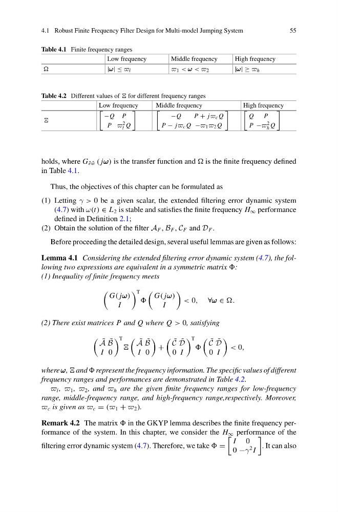
Table 4.1 Finite frequency ranges
Low frequency
Middle frequency
High frequency
|ω ω ω| ≤ l
1 < ω ω ω < 2
|ω ω ω| ≥ h
Table 4.2 Different values of for different frequency ranges
Low frequency
Middle frequency
High frequency
−Q P
P 2
l Q
−Q
P+ j c Q
P − j c Q − 1 2 Q
Q
P
P − 2
h Q
holds, where G ˜
e ˜
w ( jω ω ω) is the transfer function and is the finite frequency defined
in Table 4.1.
Thus, the objectives of this chapter can be formulated as
(1) Letting γ > 0 be a given scalar, the extended filtering error dynamic system
(4.7) with ω(t) ∈ L 2 is stable and satisfies the finite frequency H ∞ performance
defined in Definition 2.1;
(2) Obtain the solution of the filter A F , B F , C F and D F .
Before proceeding the detailed design, several useful lemmas are given as follows:
Lemma 4.1 Considering the extended filtering error dynamic system (4.7), the following two expressions are equivalent in a symmetric matrix :
(1) Inequality of finite frequency meets
G( jω ω ω)
I
T
G( jω ω ω)
I
< 0, ∀ω ω ω ∈ .
(2) There exist matrices P and Q where Q > 0, satisfying
˜
A ˜
B
I 0
T
˜
A ˜
B
I 0
+
˜
C ˜
D
0 I
T
˜
C ˜
D
0 I
< 0,
where ω ω ω, and represent the frequency information. The specific values of different
frequency ranges and performances are demonstrated in Table 4.2.
l , 1 , 2 , and h are the given finite frequency ranges for low-frequency
range, middle-frequency range, and high-frequency range,respectively. Moreover,
c is given as c = ( 1 + 2 ).
Remark 4.2 The matrix in the GKYP lemma describes the finite frequency performance of the system. In this chapter, we consider the H ∞ performance of the
filtering error dynamic system (4.7). Therefore, we take =
I 0
0 −γ
2 I
. It can also
55
Table 4.1 Finite frequency ranges
Low frequency
Middle frequency
High frequency
|ω ω ω| ≤ l
1 < ω ω ω < 2
|ω ω ω| ≥ h
Table 4.2 Different values of for different frequency ranges
Low frequency
Middle frequency
High frequency
−Q P
P 2
l Q
−Q
P+ j c Q
P − j c Q − 1 2 Q
Q
P
P − 2
h Q
holds, where G ˜
e ˜
w ( jω ω ω) is the transfer function and is the finite frequency defined
in Table 4.1.
Thus, the objectives of this chapter can be formulated as
(1) Letting γ > 0 be a given scalar, the extended filtering error dynamic system
(4.7) with ω(t) ∈ L 2 is stable and satisfies the finite frequency H ∞ performance
defined in Definition 2.1;
(2) Obtain the solution of the filter A F , B F , C F and D F .
Before proceeding the detailed design, several useful lemmas are given as follows:
Lemma 4.1 Considering the extended filtering error dynamic system (4.7), the following two expressions are equivalent in a symmetric matrix :
(1) Inequality of finite frequency meets
G( jω ω ω)
I
T
G( jω ω ω)
I
< 0, ∀ω ω ω ∈ .
(2) There exist matrices P and Q where Q > 0, satisfying
˜
A ˜
B
I 0
T
˜
A ˜
B
I 0
+
˜
C ˜
D
0 I
T
˜
C ˜
D
0 I
< 0,
where ω ω ω, and represent the frequency information. The specific values of different
frequency ranges and performances are demonstrated in Table 4.2.
l , 1 , 2 , and h are the given finite frequency ranges for low-frequency
range, middle-frequency range, and high-frequency range,respectively. Moreover,
c is given as c = ( 1 + 2 ).
Remark 4.2 The matrix in the GKYP lemma describes the finite frequency performance of the system. In this chapter, we consider the H ∞ performance of the
filtering error dynamic system (4.7). Therefore, we take =
I 0
0 −γ
2 I
. It can also