

168
9 Neural Network-Based Robust Fault Detection …
0
5
10
15
20
−6
−4
−2
0
2
4
6
t/s
The disturbance signal d(t)
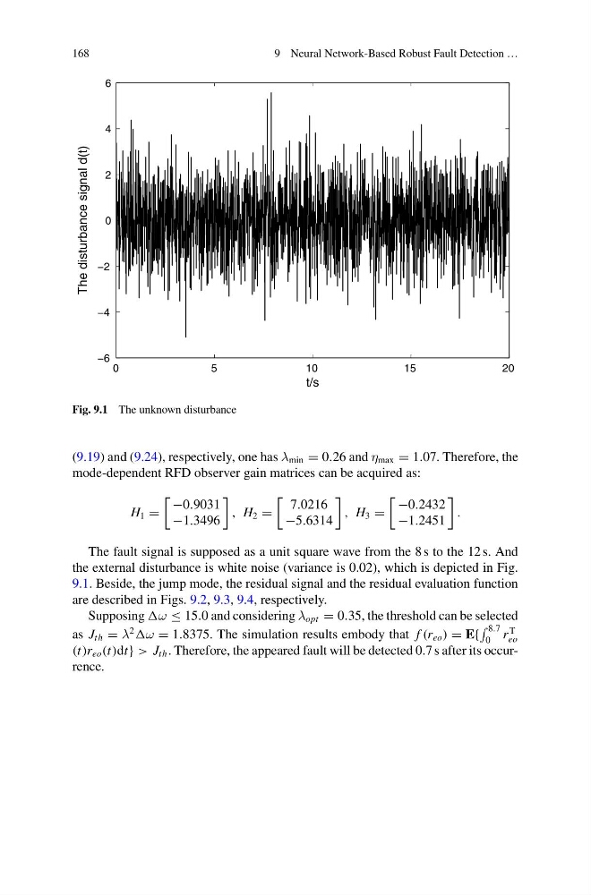
Fig. 9.1 The unknown disturbance
(9.19) and (9.24), respectively, one has λ min = 0.26 and η max = 1.07. Therefore, the
mode-dependent RFD observer gain matrices can be acquired as:
H 1 =
−0.9031
−1.3496
, H 2 =
7.0216
−5.6314
, H 3 =
−0.2432
−1.2451
.
The fault signal is supposed as a unit square wave from the 8 s to the 12 s. And
the external disturbance is white noise (variance is 0.02), which is depicted in Fig.
9.1. Beside, the jump mode, the residual signal and the residual evaluation function
are described in Figs. 9.2, 9.3, 9.4, respectively.
Supposing ≤ 15.0 and considering λ opt = 0.35, the threshold can be selected
as J th = λ
2
= 1.8375. The simulation results embody that f (r eo ) = E{
8.7
0 r
T
eo
(t)r eo (t)dt} > J th . Therefore, the appeared fault will be detected 0.7 s after its occurrence.
9 Neural Network-Based Robust Fault Detection …
0
5
10
15
20
−6
−4
−2
0
2
4
6
t/s
The disturbance signal d(t)
Fig. 9.1 The unknown disturbance
(9.19) and (9.24), respectively, one has λ min = 0.26 and η max = 1.07. Therefore, the
mode-dependent RFD observer gain matrices can be acquired as:
H 1 =
−0.9031
−1.3496
, H 2 =
7.0216
−5.6314
, H 3 =
−0.2432
−1.2451
.
The fault signal is supposed as a unit square wave from the 8 s to the 12 s. And
the external disturbance is white noise (variance is 0.02), which is depicted in Fig.
9.1. Beside, the jump mode, the residual signal and the residual evaluation function
are described in Figs. 9.2, 9.3, 9.4, respectively.
Supposing ≤ 15.0 and considering λ opt = 0.35, the threshold can be selected
as J th = λ
2
= 1.8375. The simulation results embody that f (r eo ) = E{
8.7
0 r
T
eo
(t)r eo (t)dt} > J th . Therefore, the appeared fault will be detected 0.7 s after its occurrence.