

160
9 Neural Network-Based Robust Fault Detection …
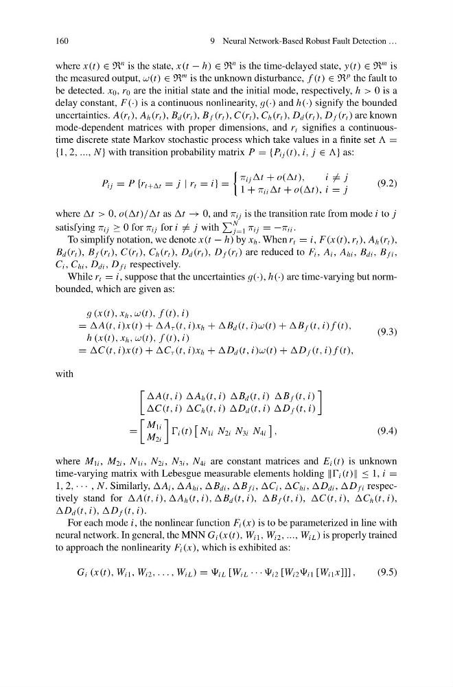
where x(t) ∈ R
n is the state, x(t − h) ∈ R
n is the time-delayed state, y(t) ∈ R
m is
the measured output, ω(t) ∈ R
m is the unknown disturbance, f (t) ∈ R
p the fault to
be detected. x 0 , r 0 are the initial state and the initial mode, respectively, h > 0 is a
delay constant, F(·) is a continuous nonlinearity, g(·) and h(·) signify the bounded
uncertainties. A(r t ), A h (r t ), B d (r t ), B f (r t ), C(r t ), C h (r t ), D d (r t ), D f (r t ) are known
mode-dependent matrices with proper dimensions, and r t signifies a continuoustime discrete state Markov stochastic process which take values in a finite set =
{1, 2, ..., N } with transition probability matrix P = {P i j (t), i, j ∈ } as:
P i j = P {r t+t = j | r t = i} =
π i j t + o((t),
i = j
1 + π ii t + o((t), i = j
(9.2)
where t > 0, o((t)//t as t → 0, and π i j is the transition rate from mode i to j
satisfying π i j ≥ 0 for π i j for i = j with
N
j=1 π i j = −π ii .
To simplify notation, we denote x(t − h) by x h . When r t = i, F(x(t), r t ), A h (r t ),
B d (r t ), B f (r t ), C(r t ), C h (r t ), D d (r t ), D f (r t ) are reduced to F i , A i , A hi , B di , B f i ,
C i , C hi , D di , D f i respectively.
While r t = i, suppose that the uncertainties g(·), h(·) are time-varying but normbounded, which are given as:
g (x(t), x h , ω(t), f (t), i)
= A(t, i)x(t) + A τ (t, i)x h + B d (t, i)ω(t) + B f (t, i) f (t),
h (x(t), x h , ω(t), f (t), i)
= C(t, i)x(t) + C τ (t, i)x h + D d (t, i)ω(t) + D f (t, i) f (t),
(9.3)
with
A(t, i) )A h (t, i) )B d (t, i) )B f (t, i)
C(t, i) )C h (t, i) )D d (t, i) )D f (t, i)
=
M 1i
M 2i
i (t)
N 1i N 2i N 3i N 4i
,
(9.4)
where M 1i , M 2i , N 1i , N 2i , N 3i , N 4i are constant matrices and E i (t) is unknown
time-varying matrix with Lebesgue measurable elements holding i (t) ≤ 1, i =
1, 2, · · · , N . Similarly, A i , A hi , B di , B f i , C i , C hi , D di , D f i respectively stand for A(t, i), ,A h (t, i), ,B d (t, i), B f (t, i), C(t, i), C h (t, i),
D d (t, i), D f (t, i).
For each mode i, the nonlinear function F i (x) is to be parameterized in line with
neural network. In general, the MNN G i (x(t), W i1 , W i2 , ..., W i L ) is properly trained
to approach the nonlinearity F i (x), which is exhibited as:
G i (x(t), W i1 , W i2 , . . . , W i L ) = i L [W i L · · · i2 [W i2 i1 [W i1 x]]] ,
(9.5)
9 Neural Network-Based Robust Fault Detection …
where x(t) ∈ R
n is the state, x(t − h) ∈ R
n is the time-delayed state, y(t) ∈ R
m is
the measured output, ω(t) ∈ R
m is the unknown disturbance, f (t) ∈ R
p the fault to
be detected. x 0 , r 0 are the initial state and the initial mode, respectively, h > 0 is a
delay constant, F(·) is a continuous nonlinearity, g(·) and h(·) signify the bounded
uncertainties. A(r t ), A h (r t ), B d (r t ), B f (r t ), C(r t ), C h (r t ), D d (r t ), D f (r t ) are known
mode-dependent matrices with proper dimensions, and r t signifies a continuoustime discrete state Markov stochastic process which take values in a finite set =
{1, 2, ..., N } with transition probability matrix P = {P i j (t), i, j ∈ } as:
P i j = P {r t+t = j | r t = i} =
π i j t + o((t),
i = j
1 + π ii t + o((t), i = j
(9.2)
where t > 0, o((t)//t as t → 0, and π i j is the transition rate from mode i to j
satisfying π i j ≥ 0 for π i j for i = j with
N
j=1 π i j = −π ii .
To simplify notation, we denote x(t − h) by x h . When r t = i, F(x(t), r t ), A h (r t ),
B d (r t ), B f (r t ), C(r t ), C h (r t ), D d (r t ), D f (r t ) are reduced to F i , A i , A hi , B di , B f i ,
C i , C hi , D di , D f i respectively.
While r t = i, suppose that the uncertainties g(·), h(·) are time-varying but normbounded, which are given as:
g (x(t), x h , ω(t), f (t), i)
= A(t, i)x(t) + A τ (t, i)x h + B d (t, i)ω(t) + B f (t, i) f (t),
h (x(t), x h , ω(t), f (t), i)
= C(t, i)x(t) + C τ (t, i)x h + D d (t, i)ω(t) + D f (t, i) f (t),
(9.3)
with
A(t, i) )A h (t, i) )B d (t, i) )B f (t, i)
C(t, i) )C h (t, i) )D d (t, i) )D f (t, i)
=
M 1i
M 2i
i (t)
N 1i N 2i N 3i N 4i
,
(9.4)
where M 1i , M 2i , N 1i , N 2i , N 3i , N 4i are constant matrices and E i (t) is unknown
time-varying matrix with Lebesgue measurable elements holding i (t) ≤ 1, i =
1, 2, · · · , N . Similarly, A i , A hi , B di , B f i , C i , C hi , D di , D f i respectively stand for A(t, i), ,A h (t, i), ,B d (t, i), B f (t, i), C(t, i), C h (t, i),
D d (t, i), D f (t, i).
For each mode i, the nonlinear function F i (x) is to be parameterized in line with
neural network. In general, the MNN G i (x(t), W i1 , W i2 , ..., W i L ) is properly trained
to approach the nonlinearity F i (x), which is exhibited as:
G i (x(t), W i1 , W i2 , . . . , W i L ) = i L [W i L · · · i2 [W i2 i1 [W i1 x]]] ,
(9.5)