

112
6 Robust Fault Detection for Multi-model Jumping System
Mode 1:
A 1 =
1.9 4.8
−1.8 −2.8
, A h1 =
−0.2 0.3
−0.1 −0.2
, B 1 =
0.5
0.3
C 1 =
1
1
, C h1 =
0.2
0.2
, B f 1 =
3.3
3.2
, D f 1 =
1.5
,
B d1 =
0.3
0.3
, D d1 =
0.4
, M 1 =
0
0
, N 1 = [0 0];
Mode 2:
A 2 =
−4.6 −1.3
2.8 −1.3
, A h2 =
−0.2 0.3
−0.4 −0.2
, B 2 =
0.4
0.3
,
C 2 =
0.8
1
, C h2 =
0.2
0.4
, B f 2 =
−1.7
1.8
, D f 2 =
3.5
,
B d2 =
0.4
0.6
, D d2 =
0.4
, M 2 =
0
0
, N 2 = [0 0].
Besides, the transition rate matrix is given as:
=
−3 3
1 −1
.
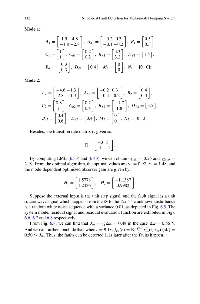
By computing LMIs (6.33) and (6.43), we can obtain γ 1min = 0.25 and γ 2max =
2.19. From the optimal algorithm, the optimal values are γ 1 = 0.92, γ 2 = 1.48, and
the mode-dependent optimized observer gain are given by:
H 1 =
1.5778
1.2436
, H 2 =
−1.1387
0.9982
.
Suppose the external input is the unit step signal, and the fault signal is a unit
square wave signal which happens from the 8s to the 12s. The unknown disturbance
is a random white noise sequence with a variance 0.01, as depicted in Fig. 6.5. The
system mode, residual signal and residual evaluation function are exhibited in Figs.
6.6, 6.7 and 6.8 respectively.
From Fig. 6.8, we can find that J th = γ
2
1 ω = 0.48 in the case ω = 0.56 V.
And we can further conclude that, when t = 9.1s, f eo (r ) = E{
9.1
0 r
T
eo (t) r eo (t)dt} =
0.50 > J th . Thus, the faults can be detected 1.1s later after the faults happen.
6 Robust Fault Detection for Multi-model Jumping System
Mode 1:
A 1 =
1.9 4.8
−1.8 −2.8
, A h1 =
−0.2 0.3
−0.1 −0.2
, B 1 =
0.5
0.3
C 1 =
1
1
, C h1 =
0.2
0.2
, B f 1 =
3.3
3.2
, D f 1 =
1.5
,
B d1 =
0.3
0.3
, D d1 =
0.4
, M 1 =
0
0
, N 1 = [0 0];
Mode 2:
A 2 =
−4.6 −1.3
2.8 −1.3
, A h2 =
−0.2 0.3
−0.4 −0.2
, B 2 =
0.4
0.3
,
C 2 =
0.8
1
, C h2 =
0.2
0.4
, B f 2 =
−1.7
1.8
, D f 2 =
3.5
,
B d2 =
0.4
0.6
, D d2 =
0.4
, M 2 =
0
0
, N 2 = [0 0].
Besides, the transition rate matrix is given as:
=
−3 3
1 −1
.
By computing LMIs (6.33) and (6.43), we can obtain γ 1min = 0.25 and γ 2max =
2.19. From the optimal algorithm, the optimal values are γ 1 = 0.92, γ 2 = 1.48, and
the mode-dependent optimized observer gain are given by:
H 1 =
1.5778
1.2436
, H 2 =
−1.1387
0.9982
.
Suppose the external input is the unit step signal, and the fault signal is a unit
square wave signal which happens from the 8s to the 12s. The unknown disturbance
is a random white noise sequence with a variance 0.01, as depicted in Fig. 6.5. The
system mode, residual signal and residual evaluation function are exhibited in Figs.
6.6, 6.7 and 6.8 respectively.
From Fig. 6.8, we can find that J th = γ
2
1 ω = 0.48 in the case ω = 0.56 V.
And we can further conclude that, when t = 9.1s, f eo (r ) = E{
9.1
0 r
T
eo (t) r eo (t)dt} =
0.50 > J th . Thus, the faults can be detected 1.1s later after the faults happen.