

5.3 Numeral Examples
91
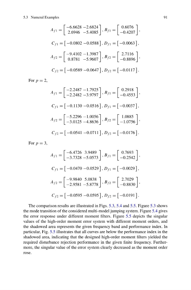
A f 1 =
−6.6628 −2.6824
2.6946 −5.4085
, B f 1 =
0.6076
−0.4207
,
C f 1 =
−0.0802 −0.0588
, D f 1 =
−0.0063
,
A f 2 =
−9.4102 −1.3987
0.8781 −5.9607
, B f 2 =
2.7116
−0.8896
,
C f 2 =
−0.0589 −0.0647
, D f 2 =
−0.0117
.
For p = 2,
A f 1 =
−2.2487 −1.7925
−2.2482 −3.9797
, B f 1 =
0.2918
−0.4553
,
C f 1 =
−0.1130 −0.0516
, D f 1 =
−0.0037
,
A f 2 =
−5.2296 −1.0056
−3.0125 −4.8636
, B f 2 =
1.0885
−1.0756
,
C f 2 =
−0.0541 −0.0711
, D f 2 =
−0.0176
.
For p = 3,
A f 1 =
−6.4726 3.9489
−3.7328 −5.0573
, B f 1 =
0.7693
−0.2542
,
C f 1 =
−0.0470 −0.0529
, D f 1 =
−0.0029
,
A f 2 =
−9.9840 5.0838
−2.9581 −5.8778
, B f 2 =
2.7029
−0.8830
,
C f 2 =
−0.0595 −0.0595
, D f 2 =
−0.0191
.
The comparison results are illustrated in Figs. 5.3, 5.4 and 5.5. Figure 5.3 shows
the mode transition of the considered multi-model jumping system. Figure 5.4 gives
the error response under different moment filters. Figure 5.5 depicts the singular
values of the high-order moment error system with different moment orders, and
the shadowed area represents the given frequency band and performance index. In
particular, Fig. 5.5 illustrates that all curves are below the performance index in the
shadowed area, indicating that the designed high-order moment filters yielded the
required disturbance rejection performance in the given finite frequency. Furthermore, the singular value of the error system clearly decreased as the moment order
rose.
91
A f 1 =
−6.6628 −2.6824
2.6946 −5.4085
, B f 1 =
0.6076
−0.4207
,
C f 1 =
−0.0802 −0.0588
, D f 1 =
−0.0063
,
A f 2 =
−9.4102 −1.3987
0.8781 −5.9607
, B f 2 =
2.7116
−0.8896
,
C f 2 =
−0.0589 −0.0647
, D f 2 =
−0.0117
.
For p = 2,
A f 1 =
−2.2487 −1.7925
−2.2482 −3.9797
, B f 1 =
0.2918
−0.4553
,
C f 1 =
−0.1130 −0.0516
, D f 1 =
−0.0037
,
A f 2 =
−5.2296 −1.0056
−3.0125 −4.8636
, B f 2 =
1.0885
−1.0756
,
C f 2 =
−0.0541 −0.0711
, D f 2 =
−0.0176
.
For p = 3,
A f 1 =
−6.4726 3.9489
−3.7328 −5.0573
, B f 1 =
0.7693
−0.2542
,
C f 1 =
−0.0470 −0.0529
, D f 1 =
−0.0029
,
A f 2 =
−9.9840 5.0838
−2.9581 −5.8778
, B f 2 =
2.7029
−0.8830
,
C f 2 =
−0.0595 −0.0595
, D f 2 =
−0.0191
.
The comparison results are illustrated in Figs. 5.3, 5.4 and 5.5. Figure 5.3 shows
the mode transition of the considered multi-model jumping system. Figure 5.4 gives
the error response under different moment filters. Figure 5.5 depicts the singular
values of the high-order moment error system with different moment orders, and
the shadowed area represents the given frequency band and performance index. In
particular, Fig. 5.5 illustrates that all curves are below the performance index in the
shadowed area, indicating that the designed high-order moment filters yielded the
required disturbance rejection performance in the given finite frequency. Furthermore, the singular value of the error system clearly decreased as the moment order
rose.