

13.1 Catalysis
579
If there is considerable experimental error in the data, it might be difficult to
locate the asymptote in Figure 13.7 accurately. To avoid this problem, Eq. (13.1-46)
is solved for the reciprocal of the initial rate. The result is called the Lineweaver–Burk
equation: 15
1
r i
K m
k 2 [E] total [R]
+
1
k 2 [E] total
(13.1-47)
where the initial rate is denoted by r i . Data on initial rates should give a straight
line when 1/r i is plotted as a function of 1/[R]. The slope of the line is equal to
K m /k 2 [E] total , the intercept on the vertical axis is equal to 1/k 2 [E] total , and the intercept
on the horizontal axis is equal to −1/K m . Note the resemblance of this plot to the linear
plot of the Langmuir isotherm in Figure 13.3.
Exercise 13.11
Show that the intercept of the Lineweaver–Burk plot on the horizontal axis is equal to −1/K m .
E X A M P L E 13.5
The following data were gathered for the myosin-catalyzed hydrolysis of ATP at 25 ◦ C and
pH 7.0:
[ATP]/µmol L −1 initial rate/µmol L −1 s −1
7.5
0.067
12.5
0.095
20.0
0.119
43.5
0.149
62.5
0.185
155.0
0.191
320.0
0.195
Determine the value of the Michaelis–Menten constant.
Solution
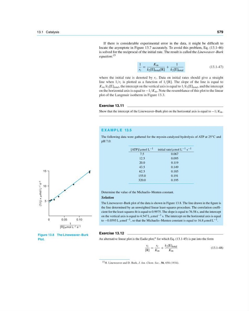
The Lineweaver–Burk plot of the data is shown in Figure 13.8. The line drawn in the figure is
the line determined by an unweighted linear least-squares procedure. The correlation coefficient for the least-squares fit is equal to 0.9975. The slope is equal to 76.58 s, and the intercept
on the vertical axis is equal to 4.547 L µmol −1 s. The intercept on the horizontal axis is equal
to −0.0595 L µmol −1 , so that the Michaelis–Menten constant is equal to 16.8 µmol L −1 .
15
10
5
0
0.05
0.10
(1/r
i ) ×
mol L –1
s –1
1
[R]/mol L –1 s –1
Figure 13.8 The Lineweaver–Burk
Plot.
Exercise 13.12
An alternative linear plot is the Eadie plot, a for which Eq. (13.1-45) is put into the form
r i
[R]
r i
K m
+
k 2 [E] total
K m
(13.1-48)
15 H. Lineweaver and D. Burk, J. Am. Chem. Soc., 56, 658 (1934).