

11.2 Forward Reactions with One Reactant
497
The Method of Initial Rates
In this method we compare data directly with the rate law instead of with an integrated
rate law. The reaction is followed for a short time ∆t during which there is a change
∆[A] in the concentration of a reactant, A:
∆[A] [A] ∆t − [A] 0
(11.2-22)
The time ∆t must be short enough that ∆[A] is much smaller than [A]. The method
has the advantage that the reverse reaction is almost certain to be negligible. The initial
rate is approximated by a quotient of finite differences:
r initial −
1
a
d[A]
dt
≈ −
1
a
∆[A]
∆t
(11.2-23)
where a is the stoichiometric coefficient of the reactant A. If there is only one reactant
and if the rate law corresponds to order α, the initial rate corresponds to Eq. (11.1-8):
r initial −
1
a
d[A]
dt
k f [A]
α
0
(11.2-24)
where [A] 0 is the initial concentration of the reactant A. We take the natural logarithm
of both sides of this equation
ln(r initial ) ln(k f ) + αln([A] 0 )
(11.2-25)
To determine the order and the rate constant, one carries out several experiments
at the same temperature but with different values of [A] 0 . A plot of the logarithm of
the initial rate as a function of the logarithm of the initial concentration is constructed
and a linear least-squares fit is performed. The slope of the line fitting the data points
is the order of the reaction, and the intercept is the logarithm of the rate constant.
A modification to the foregoing method would be to run the experiment over a longer
period of time and then to determine the value of ∆[A]/∆t and the value of [A] at
different times and to use these values in a fit to Eq. (11.2-25).
25
29
28
27
26
24
In(initial concentration)
In(initial rate)
23
22
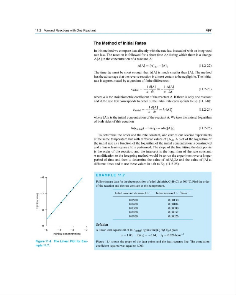
Figure 11.4 The Linear Plot for Example 11.7.
E X A M P L E 11.7
Following are data for the decomposition of ethyl chloride, C 2 H 5 Cl, at 500 ◦ C. Find the order
of the reaction and the rate constant at this temperature.
Initial concentration /mol L −1 Initial rate /mol L −1 hour −1
0.0500
0.00130
0.0400
0.00104
0.0300
0.00080
0.0200
0.00052
0.0100
0.00026
Solution
A linear least-squares fit of ln(r initial ) against ln([C 2 H 5 Cl] 0 ) gives
α 1.00, ln(k f ) −3.64, k f 0.026 hour −1
Figure 11.4 shows the graph of the data points and the least-squares line. The correlation
coefficient squared was equal to 1.000.