11.2 Forward Reactions with One Reactant
495
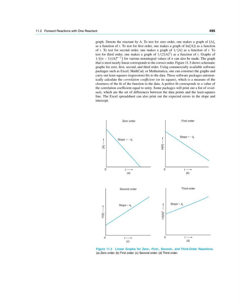
graph. Denote the reactant by A. To test for zero order, one makes a graph of [A] t
as a function of t. To test for first order, one makes a graph of ln([A]) as a function
of t. To test for second order, one makes a graph of 1/ [A] as a function of t. To
test for third order, one makes a graph of 1/(2 [A]
2 ) as a function of t. Graphs of
1/
(n − 1) [A]
n−1
for various nonintegral values of n can also be made. The graph
that is most nearly linear corresponds to the correct order. Figure 11.3 shows schematic
graphs for zero, first, second, and third order. Using commercially available software
packages such as Excel, MathCad, or Mathematica, one can construct the graphs and
carry out least-squares (regression) fits to the data. These software packages automatically calculate the correlation coefficient (or its square), which is a measure of the
closeness of the fit of the function to the data. A perfect fit corresponds to a value of
the correlation coefficient equal to unity. Some packages will print out a list of residuals, which are the set of differences between the data points and the least-squares
line. The Excel spreadsheet can also print out the expected errors in the slope and
intercept.
Slope 52k f
0
(a)
Zero order
[A]
t
Slope 5 k f
0
(c)
Second order
1/[A]
t
Slope 5 k f
0
(d)
Third order
1/2[A] 2
t
Slope 52k f
0
(b)
First order
In[A]
t
Figure 11.3 Linear Graphs for Zero-, First-, Second-, and Third-Order Reactions.
(a) Zero order. (b) First order. (c) Second order. (d) Third order.