

9.3 The Velocity Probability Distribution
399
This must agree with the macroscopic energy of a dilute gas in Eq. (9.3-24), so that
N
3m
2b
3
2
N k B T
(9.3-30)
so that
b m/k B T
(9.3-31)
The normalized probability distribution for the x component of the velocity is now
f(v x )
m
2πk B T
1/2
e −mv 2
x /2k B T
(9.3-32)
We have derived this distribution for particles without rotation or vibration, but we now
assert that rotation, vibration, and electronic motion occur independently of translation
(the only motion of structureless particles) so that we can use this distribution for
the translational motion of any molecules in a dilute gas. The normalized probability
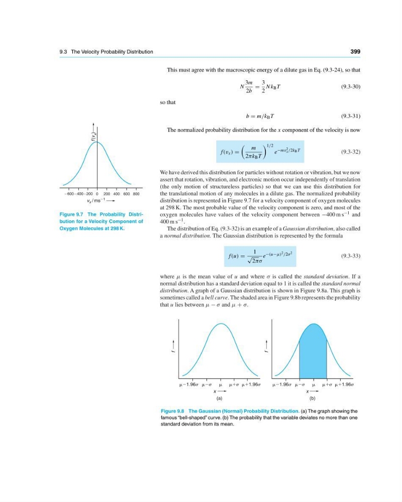
distribution is represented in Figure 9.7 for a velocity component of oxygen molecules
at 298 K. The most probable value of the velocity component is zero, and most of the
oxygen molecules have values of the velocity component between −400 m s −1 and
400 m s −1 .
260024002200
200 400 600 800
0
v x / ms 21
f (v
x
)
Figure 9.7 The Probability Distribution for a Velocity Component of
Oxygen Molecules at 298 K.
The distribution of Eq. (9.3-32) is an example of a Gaussian distribution, also called
a normal distribution. The Gaussian distribution is represented by the formula
f(u)
1
√
2πσ
e −(u−µ) 2 /2σ 2
(9.3-33)
where µ is the mean value of u and where σ is called the standard deviation. If a
normal distribution has a standard deviation equal to 1 it is called the standard normal
distribution. A graph of a Gaussian distribution is shown in Figure 9.8a. This graph is
sometimes called a bell curve. The shaded area in Figure 9.8b represents the probability
that u lies between µ − σ and µ + σ.
f
(b)
(a)
f
m21.96s
m
m 1 1.96s
x
m2s
m1s
m21.96s
m
m 1 1.96s
x
m2s
m1s
Figure 9.8 The Gaussian (Normal) Probability Distribution. (a) The graph showing the
famous “bell-shaped” curve. (b) The probability that the variable deviates no more than one
standard deviation from its mean.
399
This must agree with the macroscopic energy of a dilute gas in Eq. (9.3-24), so that
N
3m
2b
3
2
N k B T
(9.3-30)
so that
b m/k B T
(9.3-31)
The normalized probability distribution for the x component of the velocity is now
f(v x )
m
2πk B T
1/2
e −mv 2
x /2k B T
(9.3-32)
We have derived this distribution for particles without rotation or vibration, but we now
assert that rotation, vibration, and electronic motion occur independently of translation
(the only motion of structureless particles) so that we can use this distribution for
the translational motion of any molecules in a dilute gas. The normalized probability
distribution is represented in Figure 9.7 for a velocity component of oxygen molecules
at 298 K. The most probable value of the velocity component is zero, and most of the
oxygen molecules have values of the velocity component between −400 m s −1 and
400 m s −1 .
260024002200
200 400 600 800
0
v x / ms 21
f (v
x
)
Figure 9.7 The Probability Distribution for a Velocity Component of
Oxygen Molecules at 298 K.
The distribution of Eq. (9.3-32) is an example of a Gaussian distribution, also called
a normal distribution. The Gaussian distribution is represented by the formula
f(u)
1
√
2πσ
e −(u−µ) 2 /2σ 2
(9.3-33)
where µ is the mean value of u and where σ is called the standard deviation. If a
normal distribution has a standard deviation equal to 1 it is called the standard normal
distribution. A graph of a Gaussian distribution is shown in Figure 9.8a. This graph is
sometimes called a bell curve. The shaded area in Figure 9.8b represents the probability
that u lies between µ − σ and µ + σ.
f
(b)
(a)
f
m21.96s
m
m 1 1.96s
x
m2s
m1s
m21.96s
m
m 1 1.96s
x
m2s
m1s
Figure 9.8 The Gaussian (Normal) Probability Distribution. (a) The graph showing the
famous “bell-shaped” curve. (b) The probability that the variable deviates no more than one
standard deviation from its mean.