

394
9 Gas Kinetic Theory: The Molecular Theory of Dilute Gases at Equilibrium
b. Construct a graph of the position of the particle as a
function of time for m 1.00 kg, f 1.00 kg s −1 ,
x 0 0, and v 0 10.0 m s −1 .
9.5 An object is propelled upward at the surface of the earth with
an initial speed of 10.0 m s −1 . Ignoring air resistance, find
the maximum height of the object above its starting point.
9.6 An object with mass 0.100 kg slides down a frictionless
surface of some arbitrary shape near the surface of the earth.
If it starts with zero speed, find its speed when it is at a
location 0.250 m lower in altitude than its initial position,
and show that this is independent of the shape of the
surface.
9.3
The Velocity Probability Distribution
If a system obeys classical mechanics, averaging over molecular states means averaging over molecular coordinates and momenta. Coordinates and momenta vary continuously, so we must integrate over their possible values instead of summing over discrete
energies as in Eq. (9.2-19). Consider a quantity u that can take on any value between
u 1 and u 2 . We define a probability distribution f (u) such that
The probability that u lies
between u and u + du
f (u
)du
(9.3-1)
where du is an infinitesimal range of values of u and where u is some value of u.
The probability distribution f (u) is a probability per unit length on the u axis, and we
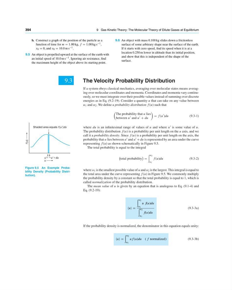
call it a probability density. Since f (u) is a probability per unit length on the axis, the
probability that u lies between u and u + du is represented by an area under the curve
representing f (u) as shown schematically in Figure 9.5.
Shaded area equals f (u' )du
f (u)
u'
u' 1du
u
Figure 9.5 An Example Probability Density (Probability Distribution).
The total probability is equal to the integral
total probability
u 2
u 1
f (u)du
(9.3-2)
where u 1 is the smallest possible value of u and u 2 is the largest. This integral is equal to
the total area under the curve representing f (u) in Figure 9.5. We commonly multiply
the probability density by a constant so that the total probability is equal to 1, which is
called normalization of the probability distribution.
The mean value of u is given by an equation that is analogous to Eq. (9.1-4) and
Eq. (9.2-19):
u
u 2
u 1
u f(u)du
u 2
u 1
f(u)du
(9.3-3a)
If the probability density is normalized, the denominator in this equation equals unity:
u
u 2
u 1
uf (u)du ( f normalized)
(9.3-3b)
9 Gas Kinetic Theory: The Molecular Theory of Dilute Gases at Equilibrium
b. Construct a graph of the position of the particle as a
function of time for m 1.00 kg, f 1.00 kg s −1 ,
x 0 0, and v 0 10.0 m s −1 .
9.5 An object is propelled upward at the surface of the earth with
an initial speed of 10.0 m s −1 . Ignoring air resistance, find
the maximum height of the object above its starting point.
9.6 An object with mass 0.100 kg slides down a frictionless
surface of some arbitrary shape near the surface of the earth.
If it starts with zero speed, find its speed when it is at a
location 0.250 m lower in altitude than its initial position,
and show that this is independent of the shape of the
surface.
9.3
The Velocity Probability Distribution
If a system obeys classical mechanics, averaging over molecular states means averaging over molecular coordinates and momenta. Coordinates and momenta vary continuously, so we must integrate over their possible values instead of summing over discrete
energies as in Eq. (9.2-19). Consider a quantity u that can take on any value between
u 1 and u 2 . We define a probability distribution f (u) such that
The probability that u lies
between u and u + du
f (u
)du
(9.3-1)
where du is an infinitesimal range of values of u and where u is some value of u.
The probability distribution f (u) is a probability per unit length on the u axis, and we
call it a probability density. Since f (u) is a probability per unit length on the axis, the
probability that u lies between u and u + du is represented by an area under the curve
representing f (u) as shown schematically in Figure 9.5.
Shaded area equals f (u' )du
f (u)
u'
u' 1du
u
Figure 9.5 An Example Probability Density (Probability Distribution).
The total probability is equal to the integral
total probability
u 2
u 1
f (u)du
(9.3-2)
where u 1 is the smallest possible value of u and u 2 is the largest. This integral is equal to
the total area under the curve representing f (u) in Figure 9.5. We commonly multiply
the probability density by a constant so that the total probability is equal to 1, which is
called normalization of the probability distribution.
The mean value of u is given by an equation that is analogous to Eq. (9.1-4) and
Eq. (9.2-19):
u
u 2
u 1
u f(u)du
u 2
u 1
f(u)du
(9.3-3a)
If the probability density is normalized, the denominator in this equation equals unity:
u
u 2
u 1
uf (u)du ( f normalized)
(9.3-3b)