

7.6 The Temperature Dependence of Chemical Equilibrium. The Principle of Le Châtelier
337
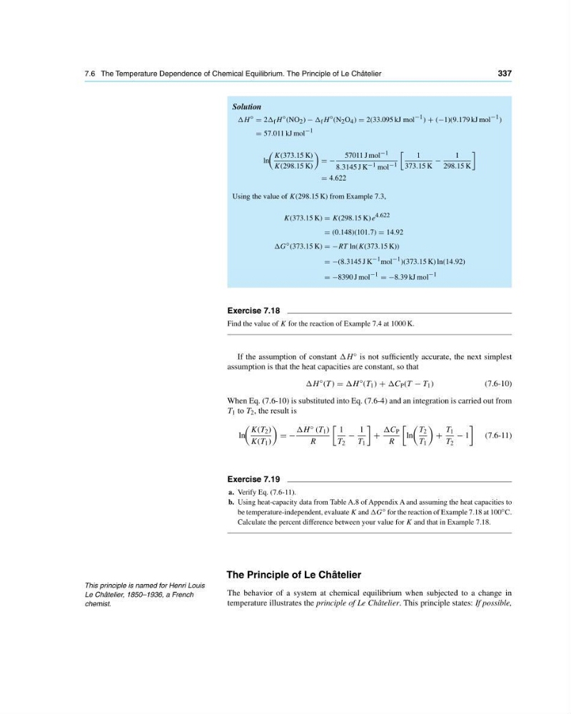
Solution
∆H ◦ 2∆ f H ◦ (NO 2 ) − ∆ f H ◦ (N 2 O 4 ) 2(33.095 kJ mol −1 ) + (−1)(9.179 kJ mol −1 )
57.011 kJ mol −1
ln
K(373.15 K)
K(298.15 K)
−
57011 J mol −1
8.3145 J K −1 mol −1
1
373.15 K
−
1
298.15 K
4.622
Using the value of K(298.15 K) from Example 7.3,
K(373.15 K) K(298.15 K) e 4.622
(0.148)(101.7) 14.92
∆G ◦ (373.15 K) −RT ln(K(373.15 K))
−(8.3145 J K −1 mol −1 )(373.15 K) ln(14.92)
−8390 J mol −1 −8.39 kJ mol −1
Exercise 7.18
Find the value of K for the reaction of Example 7.4 at 1000 K.
If the assumption of constant ∆H ◦ is not sufficiently accurate, the next simplest
assumption is that the heat capacities are constant, so that
∆H
◦ (T ) ∆H
◦ (T 1 ) + ∆C P (T − T 1 )
(7.6-10)
When Eq. (7.6-10) is substituted into Eq. (7.6-4) and an integration is carried out from
T 1 to T 2 , the result is
ln
K(T 2 )
K(T 1 )
−
∆H ◦ (T 1 )
R
1
T 2
−
1
T 1
+
∆C P
R
ln
T 2
T 1
+
T 1
T 2
− 1
(7.6-11)
Exercise 7.19
a. Verify Eq. (7.6-11).
b. Using heat-capacity data from Table A.8 of Appendix A and assuming the heat capacities to
be temperature-independent, evaluate K and ∆G ◦ for the reaction of Example 7.18 at 100 ◦ C.
Calculate the percent difference between your value for K and that in Example 7.18.
This principle is named for Henri Louis
Le Châtelier, 1850–1936, a French
chemist.
The Principle of Le Châtelier
The behavior of a system at chemical equilibrium when subjected to a change in
temperature illustrates the principle of Le Châtelier. This principle states: If possible,
337
Solution
∆H ◦ 2∆ f H ◦ (NO 2 ) − ∆ f H ◦ (N 2 O 4 ) 2(33.095 kJ mol −1 ) + (−1)(9.179 kJ mol −1 )
57.011 kJ mol −1
ln
K(373.15 K)
K(298.15 K)
−
57011 J mol −1
8.3145 J K −1 mol −1
1
373.15 K
−
1
298.15 K
4.622
Using the value of K(298.15 K) from Example 7.3,
K(373.15 K) K(298.15 K) e 4.622
(0.148)(101.7) 14.92
∆G ◦ (373.15 K) −RT ln(K(373.15 K))
−(8.3145 J K −1 mol −1 )(373.15 K) ln(14.92)
−8390 J mol −1 −8.39 kJ mol −1
Exercise 7.18
Find the value of K for the reaction of Example 7.4 at 1000 K.
If the assumption of constant ∆H ◦ is not sufficiently accurate, the next simplest
assumption is that the heat capacities are constant, so that
∆H
◦ (T ) ∆H
◦ (T 1 ) + ∆C P (T − T 1 )
(7.6-10)
When Eq. (7.6-10) is substituted into Eq. (7.6-4) and an integration is carried out from
T 1 to T 2 , the result is
ln
K(T 2 )
K(T 1 )
−
∆H ◦ (T 1 )
R
1
T 2
−
1
T 1
+
∆C P
R
ln
T 2
T 1
+
T 1
T 2
− 1
(7.6-11)
Exercise 7.19
a. Verify Eq. (7.6-11).
b. Using heat-capacity data from Table A.8 of Appendix A and assuming the heat capacities to
be temperature-independent, evaluate K and ∆G ◦ for the reaction of Example 7.18 at 100 ◦ C.
Calculate the percent difference between your value for K and that in Example 7.18.
This principle is named for Henri Louis
Le Châtelier, 1850–1936, a French
chemist.
The Principle of Le Châtelier
The behavior of a system at chemical equilibrium when subjected to a change in
temperature illustrates the principle of Le Châtelier. This principle states: If possible,