

5.3 Phase Equilibria in One-Component Systems
211
Exercise 5.6
Compare the molar volumes of liquid water at 100 ◦ C and water vapor at 100 ◦ C and 1.00 atm.
Assume that the water vapor is an ideal gas.
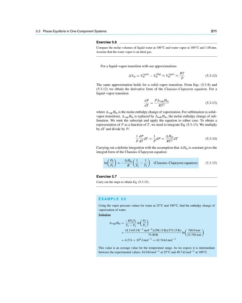
For a liquid–vapor transition with our approximations
∆V m V
(gas)
m
− V
(liq)
m
≈ V
(gas)
m
≈
RT
P
(5.3-12)
The same approximation holds for a solid–vapor transition. From Eqs. (5.3-8) and
(5.3-12) we obtain the derivative form of the Clausius–Clapeyron equation. For a
liquid–vapor transition
dP
dT
P∆ vap H m
RT 2
(5.3-13)
where ∆ vap H m is the molar enthalpy change of vaporization. For sublimation (a solid–
vapor transition), ∆ vap H m is replaced by ∆ sub H m , the molar enthalpy change of sublimation. We omit the subscript and apply the equation to either case. To obtain a
representation of P as a function of T , we need to integrate Eq. (5.3-13). We multiply
by dT and divide by P:
1
P
dP
dT
dT
1
P
dP
∆H m
RT 2 dT
(5.3-14)
Carrying out a definite integration with the assumption that ∆H m is constant gives the
integral form of the Clausius–Clapeyron equation:
ln
P 2
P 1
−
∆H m
R
1
T 2
−
1
T 1
(Clausius–Clapeyron equation)
(5.3-15)
Exercise 5.7
Carry out the steps to obtain Eq. (5.3-15).
E X A M P L E 5.5
Using the vapor pressure values for water at 25 ◦ C and 100 ◦ C, find the enthalpy change of
vaporization of water.
Solution
∆ vap H m
−RT 2 T 1
T 1 − T 2
ln
P 2
P 1
(8.3145 J K −1 mol −1 )(298.15 K)(373.15 K)
75.00 K
ln
760.0 torr
23.756 torr
4.274 × 10 4 J mol −1 42.74 kJ mol −1
This value is an average value for the temperature range. As we expect, it is intermediate
between the experimental values: 44.0 kJ mol −1 at 25 ◦ C and 40.7 kJ mol −1 at 100 ◦ C.
211
Exercise 5.6
Compare the molar volumes of liquid water at 100 ◦ C and water vapor at 100 ◦ C and 1.00 atm.
Assume that the water vapor is an ideal gas.
For a liquid–vapor transition with our approximations
∆V m V
(gas)
m
− V
(liq)
m
≈ V
(gas)
m
≈
RT
P
(5.3-12)
The same approximation holds for a solid–vapor transition. From Eqs. (5.3-8) and
(5.3-12) we obtain the derivative form of the Clausius–Clapeyron equation. For a
liquid–vapor transition
dP
dT
P∆ vap H m
RT 2
(5.3-13)
where ∆ vap H m is the molar enthalpy change of vaporization. For sublimation (a solid–
vapor transition), ∆ vap H m is replaced by ∆ sub H m , the molar enthalpy change of sublimation. We omit the subscript and apply the equation to either case. To obtain a
representation of P as a function of T , we need to integrate Eq. (5.3-13). We multiply
by dT and divide by P:
1
P
dP
dT
dT
1
P
dP
∆H m
RT 2 dT
(5.3-14)
Carrying out a definite integration with the assumption that ∆H m is constant gives the
integral form of the Clausius–Clapeyron equation:
ln
P 2
P 1
−
∆H m
R
1
T 2
−
1
T 1
(Clausius–Clapeyron equation)
(5.3-15)
Exercise 5.7
Carry out the steps to obtain Eq. (5.3-15).
E X A M P L E 5.5
Using the vapor pressure values for water at 25 ◦ C and 100 ◦ C, find the enthalpy change of
vaporization of water.
Solution
∆ vap H m
−RT 2 T 1
T 1 − T 2
ln
P 2
P 1
(8.3145 J K −1 mol −1 )(298.15 K)(373.15 K)
75.00 K
ln
760.0 torr
23.756 torr
4.274 × 10 4 J mol −1 42.74 kJ mol −1
This value is an average value for the temperature range. As we expect, it is intermediate
between the experimental values: 44.0 kJ mol −1 at 25 ◦ C and 40.7 kJ mol −1 at 100 ◦ C.