

Multiconfigurational Approach to X-ray Spectroscopy …
199
As expected, without any SOC, there is a single edge. Inclusion of 2p SOC not only
splits the spectrum into L 3 (J 2 p =
3
2
) and L 2 (J 2 p =
1
2
) edges but also leads to major
changes in spectral shape because of the mixing of states with different multiplicity.
This shows that the spin–orbit effect cannot always be modeled by simply duplicating
the spin-free spectrum and shifting the two edges away from each other. It is also
important to note that to form the correct spin–orbit states requires all three 2p orbitals
in the active space.
The 3d SOC constant is much weaker, 0.05 eV for iron, than the 2p one (8 eV).
However, taking 3d SOC into account leads to visible changes in the calculated spectrum, especially in the intensities of the two 2 p → t 2g peaks, see Fig. 8. This can be
explained by the selection rules, see Fig. 8b. Ignoring Jahn–Teller distortions, which
have only minor effects on the energy levels [71], there is triple orbital degeneracy
in the ground state. This degeneracy is lifted by spin–orbit coupling, and the lowest
spin–orbit states have different selection rules compared to the low-lying excited
states and thus generate different spectra.
3.7 Simulating X-ray Processes with Molcas
The X-ray calculations described in this chapter have almost exclusively been performed using the Molcas program [5], which is a leading program for multiconfigurational quantum chemistry. The same capabilities are also available in the open-source
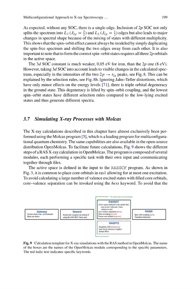
distribution OpenMolcas. To facilitate future calculations, Fig. 9 shows the different
steps of a RAS X-ray calculation in OpenMolcas. The program is composed of several
modules, each performing a specific task with their own input and communicating
together through files.
The active space is defined in the input to the RASSCF program. As shown in
Fig. 3, it is common to place core orbitals in ras1 allowing for at most one excitation.
To avoid calculating a large number of valence excited states with filled core orbitals,
core–valence separation can be invoked using the hexs keyword. To avoid that the
Fig. 9 Calculation template for X-ray simulations with the RAS method in OpenMolcas. The name
of the boxes are the names of the OpenMolcas module corresponding to the specific parameters.
The red italic text indicates specific keywords
199
As expected, without any SOC, there is a single edge. Inclusion of 2p SOC not only
splits the spectrum into L 3 (J 2 p =
3
2
) and L 2 (J 2 p =
1
2
) edges but also leads to major
changes in spectral shape because of the mixing of states with different multiplicity.
This shows that the spin–orbit effect cannot always be modeled by simply duplicating
the spin-free spectrum and shifting the two edges away from each other. It is also
important to note that to form the correct spin–orbit states requires all three 2p orbitals
in the active space.
The 3d SOC constant is much weaker, 0.05 eV for iron, than the 2p one (8 eV).
However, taking 3d SOC into account leads to visible changes in the calculated spectrum, especially in the intensities of the two 2 p → t 2g peaks, see Fig. 8. This can be
explained by the selection rules, see Fig. 8b. Ignoring Jahn–Teller distortions, which
have only minor effects on the energy levels [71], there is triple orbital degeneracy
in the ground state. This degeneracy is lifted by spin–orbit coupling, and the lowest
spin–orbit states have different selection rules compared to the low-lying excited
states and thus generate different spectra.
3.7 Simulating X-ray Processes with Molcas
The X-ray calculations described in this chapter have almost exclusively been performed using the Molcas program [5], which is a leading program for multiconfigurational quantum chemistry. The same capabilities are also available in the open-source
distribution OpenMolcas. To facilitate future calculations, Fig. 9 shows the different
steps of a RAS X-ray calculation in OpenMolcas. The program is composed of several
modules, each performing a specific task with their own input and communicating
together through files.
The active space is defined in the input to the RASSCF program. As shown in
Fig. 3, it is common to place core orbitals in ras1 allowing for at most one excitation.
To avoid calculating a large number of valence excited states with filled core orbitals,
core–valence separation can be invoked using the hexs keyword. To avoid that the
Fig. 9 Calculation template for X-ray simulations with the RAS method in OpenMolcas. The name
of the boxes are the names of the OpenMolcas module corresponding to the specific parameters.
The red italic text indicates specific keywords