

New Strategies in Modeling Electronic Structures and Properties …
133
fashion [90]. One microiteration includes three distinct steps: (1) blocking, (2) diagonalization, and (3) decimation. First, the L-orbital space is partitioned into three
subspaces: a system block, an environment block, and q exactly represented orbitals
in between represented by 4 basis functions in the case of spatial orbitals. In the
blocking step, the system and, if q = 2, the environment are enlarged by one of
the exactly represented orbitals. The many-particle basis states are defined as a tensor product of basis states of the subsystem block and the neighbouring exactlyrepresented orbital. In the second step, the Hamiltonian of the superblock (enlarged
system+enlarged environment block) is constructed and diagonalized. Usually, we
are only interested in the ground-state wave function and hence only one root of
the superblock Hamiltonian needs to be computed. In the third and last step, the
dimensionality of the enlarged system and enlarged environment blocks is reduced
to prevent the many-particle basis from growing exponentially (due to the blocking
step). The number of basis functions is reduced to a limit indicated by a parameter m.
In DMRG, this so-called renormalization step is performed in a specific way. From
the superblock wave function Ψ
SB , we calculate the many-particle reduced density
matrix of the enlarged active system block ρ
s
= Tr m e
Ψ
SB
Ψ
SB
, where m e indicate states defined on the (enlarged) environment block. This reduced density matrix
ρ
s is then diagonalized and the eigenvectors corresponding to the m largest eigenvalues form the new many-particle basis of the enlarged system block. In the final
renormalization step, all matrix representations of operators are transformed into this
new basis. Specifically, the computed transformation matrices correspond to the A
matrices of the MPS ansatz. Thus, each microiteration step optimizes exactly one
MPS matrix A and we have to sweep through the lattice to obtain an (approximate)
full representation of the MPS. After the decimation step, the algorithm starts again
with the blocking procedure, where the new system block is enlarged by one orbital,
while the new environment is reduced by one orbital. We should note that the choice
of m is crucial to find a balance between accuracy and computational cost. There is,
however, no straightforward formula that indicates the best value of m and several
calculations with different values of m are required to converge the wave function
with satisfactory accuracy.
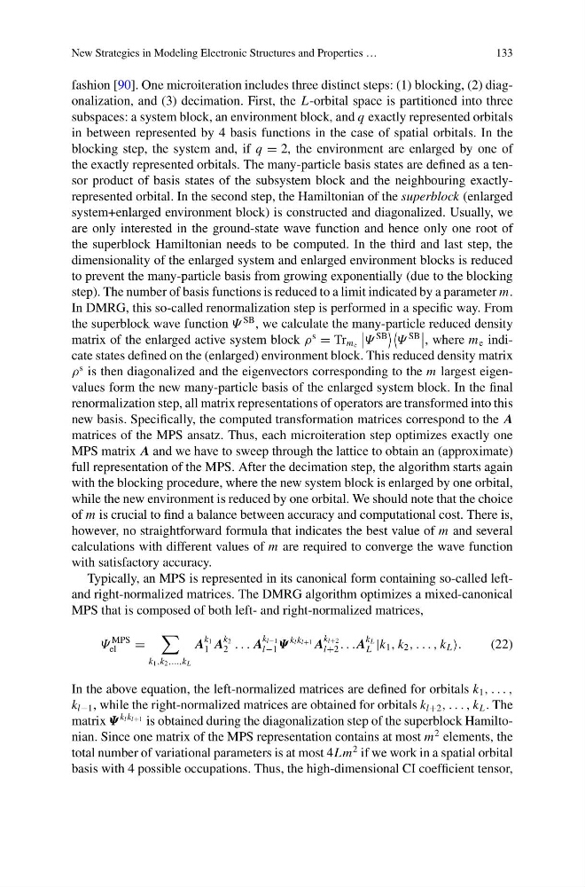
Typically, an MPS is represented in its canonical form containing so-called leftand right-normalized matrices. The DMRG algorithm optimizes a mixed-canonical
MPS that is composed of both left- and right-normalized matrices,
Ψ
MPS
el
=
k 1 ,k 2 ,...,k L
A
k 1
1 A
k 2
2 . . . A
k l−1
l−1 Ψ
k l k l+1 A
k l+2
l+2 . . .A
k L
L |k 1 , k 2 , . . . , k L .
(22)
In the above equation, the left-normalized matrices are defined for orbitals k 1 , . . . ,
k l−1 , while the right-normalized matrices are obtained for orbitals k l+2 , . . . , k L . The
matrix Ψ
k l k l+1 is obtained during the diagonalization step of the superblock Hamiltonian. Since one matrix of the MPS representation contains at most m
2 elements, the
total number of variational parameters is at most 4Lm
2 if we work in a spatial orbital
basis with 4 possible occupations. Thus, the high-dimensional CI coefficient tensor,
133
fashion [90]. One microiteration includes three distinct steps: (1) blocking, (2) diagonalization, and (3) decimation. First, the L-orbital space is partitioned into three
subspaces: a system block, an environment block, and q exactly represented orbitals
in between represented by 4 basis functions in the case of spatial orbitals. In the
blocking step, the system and, if q = 2, the environment are enlarged by one of
the exactly represented orbitals. The many-particle basis states are defined as a tensor product of basis states of the subsystem block and the neighbouring exactlyrepresented orbital. In the second step, the Hamiltonian of the superblock (enlarged
system+enlarged environment block) is constructed and diagonalized. Usually, we
are only interested in the ground-state wave function and hence only one root of
the superblock Hamiltonian needs to be computed. In the third and last step, the
dimensionality of the enlarged system and enlarged environment blocks is reduced
to prevent the many-particle basis from growing exponentially (due to the blocking
step). The number of basis functions is reduced to a limit indicated by a parameter m.
In DMRG, this so-called renormalization step is performed in a specific way. From
the superblock wave function Ψ
SB , we calculate the many-particle reduced density
matrix of the enlarged active system block ρ
s
= Tr m e
Ψ
SB
Ψ
SB
, where m e indicate states defined on the (enlarged) environment block. This reduced density matrix
ρ
s is then diagonalized and the eigenvectors corresponding to the m largest eigenvalues form the new many-particle basis of the enlarged system block. In the final
renormalization step, all matrix representations of operators are transformed into this
new basis. Specifically, the computed transformation matrices correspond to the A
matrices of the MPS ansatz. Thus, each microiteration step optimizes exactly one
MPS matrix A and we have to sweep through the lattice to obtain an (approximate)
full representation of the MPS. After the decimation step, the algorithm starts again
with the blocking procedure, where the new system block is enlarged by one orbital,
while the new environment is reduced by one orbital. We should note that the choice
of m is crucial to find a balance between accuracy and computational cost. There is,
however, no straightforward formula that indicates the best value of m and several
calculations with different values of m are required to converge the wave function
with satisfactory accuracy.
Typically, an MPS is represented in its canonical form containing so-called leftand right-normalized matrices. The DMRG algorithm optimizes a mixed-canonical
MPS that is composed of both left- and right-normalized matrices,
Ψ
MPS
el
=
k 1 ,k 2 ,...,k L
A
k 1
1 A
k 2
2 . . . A
k l−1
l−1 Ψ
k l k l+1 A
k l+2
l+2 . . .A
k L
L |k 1 , k 2 , . . . , k L .
(22)
In the above equation, the left-normalized matrices are defined for orbitals k 1 , . . . ,
k l−1 , while the right-normalized matrices are obtained for orbitals k l+2 , . . . , k L . The
matrix Ψ
k l k l+1 is obtained during the diagonalization step of the superblock Hamiltonian. Since one matrix of the MPS representation contains at most m
2 elements, the
total number of variational parameters is at most 4Lm
2 if we work in a spatial orbital
basis with 4 possible occupations. Thus, the high-dimensional CI coefficient tensor,