

5 Calibration
55
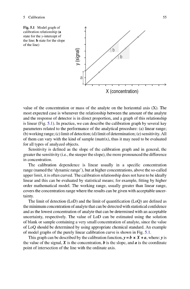
Fig. 5.1 Model graph of
calibration relationship (a
state for the y-intercept of
the line; b state for the slope
of the line)
y (signal)
X (concentration)
a
value of the concentration or mass of the analyte on the horizontal axis (X). The
most expected case is whenever the relationship between the amount of the analyte
and the response of detector is in direct proportion, and a graph of this relationship
is linear (Fig. 5.1). In practice, we can describe the calibration graph by several key
parameters related to the performance of the analytical procedure: (a) linear range;
(b) working range; (c) limit of detection; (d) limit of determination; (e) sensitivity. All
of them can vary with the kind of sample (matrix), thus it may need to be evaluated
for all types of analyzed objects.
Sensitivity is defined as the slope of the calibration graph and in general, the
greater the sensitivity (i.e., the steeper the slope), the more pronounced the difference
in concentration.
The calibration dependence is linear usually in a specific concentration
range (named the ‘dynamic range’), but at higher concentrations, above the so-called
upper limit, it is often curved. The calibration relationship does not have to be ideally
linear and this can be evaluated by statistical means; for example, fitting by higher
order mathematical model. The working range, usually greater than linear range,
covers the concentration range where the results can be given with acceptable uncertainty.
The limit of detection (LoD) and the limit of quantification (LoQ) are defined as
the minimum concentration of analyte that can be detected with statistical confidence
and as the lowest concentration of analyte that can be determined with an acceptable
uncertainty, respectively. The value of LoD can be estimated using the solution
of blank or sample containing a very small concentration of analyte, since the value
of LoQ should be determined by using appropriate chemical standard. An example
of model graphs of the purely linear calibration curve is shown in Fig. 5.1.
This graph can be described by the calibration function, y = b × X + a, where: y is
the value of the signal, X is the concentration, b is the slope, and a is the coordinate
point of intersection of the line with the ordinate axis.
55
Fig. 5.1 Model graph of
calibration relationship (a
state for the y-intercept of
the line; b state for the slope
of the line)
y (signal)
X (concentration)
a
value of the concentration or mass of the analyte on the horizontal axis (X). The
most expected case is whenever the relationship between the amount of the analyte
and the response of detector is in direct proportion, and a graph of this relationship
is linear (Fig. 5.1). In practice, we can describe the calibration graph by several key
parameters related to the performance of the analytical procedure: (a) linear range;
(b) working range; (c) limit of detection; (d) limit of determination; (e) sensitivity. All
of them can vary with the kind of sample (matrix), thus it may need to be evaluated
for all types of analyzed objects.
Sensitivity is defined as the slope of the calibration graph and in general, the
greater the sensitivity (i.e., the steeper the slope), the more pronounced the difference
in concentration.
The calibration dependence is linear usually in a specific concentration
range (named the ‘dynamic range’), but at higher concentrations, above the so-called
upper limit, it is often curved. The calibration relationship does not have to be ideally
linear and this can be evaluated by statistical means; for example, fitting by higher
order mathematical model. The working range, usually greater than linear range,
covers the concentration range where the results can be given with acceptable uncertainty.
The limit of detection (LoD) and the limit of quantification (LoQ) are defined as
the minimum concentration of analyte that can be detected with statistical confidence
and as the lowest concentration of analyte that can be determined with an acceptable
uncertainty, respectively. The value of LoD can be estimated using the solution
of blank or sample containing a very small concentration of analyte, since the value
of LoQ should be determined by using appropriate chemical standard. An example
of model graphs of the purely linear calibration curve is shown in Fig. 5.1.
This graph can be described by the calibration function, y = b × X + a, where: y is
the value of the signal, X is the concentration, b is the slope, and a is the coordinate
point of intersection of the line with the ordinate axis.