

6.1 Second-Order Diagrams
79
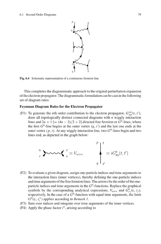
Fig. 6.4 Schematic representation of a continuous fermion line
This completes the diagrammatic approach to the original perturbation expansion
of the electron propagator. The diagrammatic formulation can be cast in the following
set of diagram rules:
Feynman Diagram Rules for the Electron Propagator
(F1) To generate the nth order contribution to the electron propagator, G
(n)
pq (t, t
),
draw all topologically distinct connected diagrams with n wiggly interaction
lines and 2n + 1 [= (4n − 2)/2 + 2] directed free fermion or G
0 -lines, where
the first G
0 -line begins at the outer vertex (q, t
) and the last one ends at the
outer vertex ( p, t). At any wiggly interaction line, two G
0 -lines begin and two
lines end, as depicted in the graph below:
(F2) To evaluate a given diagram, assign one-particle indices and time arguments to
the interaction lines (inner vertices), thereby defining the one-particle indices
and time arguments of the free fermion lines. The arrows fix the order of the oneparticle indices and time arguments in the G
0 -functions. Replace the graphical
symbols by the corresponding analytical expressions, V uvrs and G
0
rs (t i , t j ),
respectively. In the case of a G
0 -function with equal time arguments, the limit
G
0
(t i , t
+
i ) applies according to Remark 1.
(F3) Sum over indices and integrate over time arguments of the inner vertices.
(F4) Apply the phase factor i
n , arising according to
79
Fig. 6.4 Schematic representation of a continuous fermion line
This completes the diagrammatic approach to the original perturbation expansion
of the electron propagator. The diagrammatic formulation can be cast in the following
set of diagram rules:
Feynman Diagram Rules for the Electron Propagator
(F1) To generate the nth order contribution to the electron propagator, G
(n)
pq (t, t
),
draw all topologically distinct connected diagrams with n wiggly interaction
lines and 2n + 1 [= (4n − 2)/2 + 2] directed free fermion or G
0 -lines, where
the first G
0 -line begins at the outer vertex (q, t
) and the last one ends at the
outer vertex ( p, t). At any wiggly interaction line, two G
0 -lines begin and two
lines end, as depicted in the graph below:
(F2) To evaluate a given diagram, assign one-particle indices and time arguments to
the interaction lines (inner vertices), thereby defining the one-particle indices
and time arguments of the free fermion lines. The arrows fix the order of the oneparticle indices and time arguments in the G
0 -functions. Replace the graphical
symbols by the corresponding analytical expressions, V uvrs and G
0
rs (t i , t j ),
respectively. In the case of a G
0 -function with equal time arguments, the limit
G
0
(t i , t
+
i ) applies according to Remark 1.
(F3) Sum over indices and integrate over time arguments of the inner vertices.
(F4) Apply the phase factor i
n , arising according to