

56
4 Perturbation Theory for the Electron Propagator
E 0 == 0 | ˆ
H | 0
=E
(0)
0 + + 0 | ˆ
H I | 0 +
∞
n=1
0 | ˆ
H I
ˆ
Q 0
E
(0)
0 − ˆ
H 0
E
(0)
0 − E 0 + ˆ
H I
n
| 0
(4.61)
where ˆ
Q 0 = ˆ
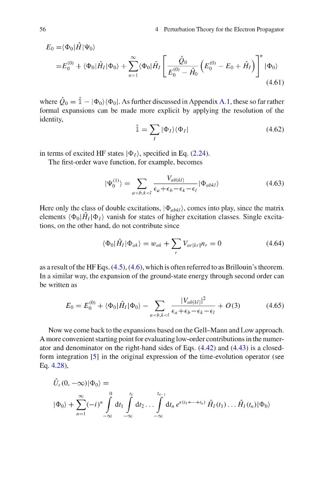
1 − | 0 0 |. As further discussed in Appendix A.1, these so far rather
formal expansions can be made more explicit by applying the resolution of the
identity,
ˆ
1 =
I
| I I |
(4.62)
in terms of excited HF states | I , specified in Eq. (2.24).
The first-order wave function, for example, becomes
|
(1)
0 =
a
a + b − k − l
| abkl
(4.63)
Here only the class of double excitations, | abkl , comes into play, since the matrix
elements 0 | ˆ
H I | I vanish for states of higher excitation classes. Single excitations, on the other hand, do not contribute since
0 | ˆ
H I | ak = w ak +
r
V ar[kr] n r = 0
(4.64)
as a result of the HF Eqs. (4.5), (4.6), which is often referred to as Brillouin’s theorem.
In a similar way, the expansion of the ground-state energy through second order can
be written as
E 0 = E
(0)
0 + + 0 | ˆ
H I | 0 −
a
2
a + b − k − l
+ O(3)
(4.65)
Now we come back to the expansions based on the Gell–Mann and Low approach.
A more convenient starting point for evaluating low-order contributions in the numerator and denominator on the right-hand sides of Eqs. (4.42) and (4.43) is a closedform integration [5] in the original expression of the time-evolution operator (see
Eq. 4.28),
ˆ
U (0, −∞)| 0 =
| 0 +
∞
n=1
(−i)
n
0
−∞
dt 1
t 1
−∞
dt 2 . . .
t n−1
−∞
dt n e
(t 1 +···+t n ) ˆ
H I (t 1 ) . . . ˆ
H I (t n )| 0
4 Perturbation Theory for the Electron Propagator
E 0 == 0 | ˆ
H | 0
=E
(0)
0 + + 0 | ˆ
H I | 0 +
∞
n=1
0 | ˆ
H I
ˆ
Q 0
E
(0)
0 − ˆ
H 0
E
(0)
0 − E 0 + ˆ
H I
n
| 0
(4.61)
where ˆ
Q 0 = ˆ
1 − | 0 0 |. As further discussed in Appendix A.1, these so far rather
formal expansions can be made more explicit by applying the resolution of the
identity,
ˆ
1 =
I
| I I |
(4.62)
in terms of excited HF states | I , specified in Eq. (2.24).
The first-order wave function, for example, becomes
|
(1)
0 =
a
a + b − k − l
| abkl
(4.63)
Here only the class of double excitations, | abkl , comes into play, since the matrix
elements 0 | ˆ
H I | I vanish for states of higher excitation classes. Single excitations, on the other hand, do not contribute since
0 | ˆ
H I | ak = w ak +
r
V ar[kr] n r = 0
(4.64)
as a result of the HF Eqs. (4.5), (4.6), which is often referred to as Brillouin’s theorem.
In a similar way, the expansion of the ground-state energy through second order can
be written as
E 0 = E
(0)
0 + + 0 | ˆ
H I | 0 −
a
2
a + b − k − l
+ O(3)
(4.65)
Now we come back to the expansions based on the Gell–Mann and Low approach.
A more convenient starting point for evaluating low-order contributions in the numerator and denominator on the right-hand sides of Eqs. (4.42) and (4.43) is a closedform integration [5] in the original expression of the time-evolution operator (see
Eq. 4.28),
ˆ
U (0, −∞)| 0 =
| 0 +
∞
n=1
(−i)
n
0
−∞
dt 1
t 1
−∞
dt 2 . . .
t n−1
−∞
dt n e
(t 1 +···+t n ) ˆ
H I (t 1 ) . . . ˆ
H I (t n )| 0