

248
16 Algebraic Propagator Methods
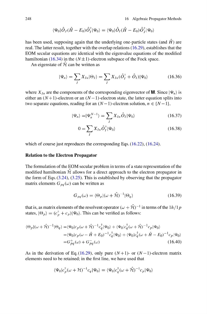
0 | ˆ
O J ( ˆ
H − E 0 ) ˆ
O
†
I | 0 = = 0 | ˆ
O I ( ˆ
H − E 0 ) ˆ
O
†
J | 0
has been used, supposing again that the underlying one-particle states (and ˆ
H ) are
real. The latter result, together with the overlap relations (16.29), establishes that the
EOM secular equations are identical with the eigenvalue equations of the modified
hamiltonian (16.34) in the (N ±1)-electron subspace of the Fock space.
An eigenstate of ˆ
H can be written as
| n =
I
X I n | I =
I
X I n ( ˆ
O
†
I + ˆ
O I )| 0
(16.36)
where X I n are the components of the corresponding eigenvector of M. Since | n is
either an (N +1)-electron or an (N −1)-electron state, the latter equation splits into
two separate equations, reading for an (N −1)-electron solution, n ∈ {N −1},
| n =|
N −1
n
=
I
X I n ˆ
O I | 0
(16.37)
0 =
I
X I n ˆ
O
†
I | 0
(16.38)
which of course just reproduces the corresponding Eqs. (16.22), (16.24).
Relation to the Electron Propagator
The formulation of the EOM secular problem in terms of a state representation of the
modified hamiltonian ˆ
H allows for a direct approach to the electron propagator in
the form of Eqs. (3.24), (3.25). This is established by observing that the propagator
matrix elements G pq (ω) can be written as
G pq (ω) = = p |(ω + ˆ
H)
−1
| q
(16.39)
that is, as matrix elements of the resolvent operator (ω + ˆ
H)
−1 in terms of the 1h/1 p
states, | p = (c
†
p + c p )| 0 . This can be verified as follows:
p |(ω + ˆ
H) −1 | q == 0 |c p (ω + ˆ
H) −1 c
†
q | 0 + + 0 |c
†
q (ω + ˆ
H) −1 c p | 0
== 0 |c p (ω − ˆ
H + E 0 ) −1 c
†
q | 0 + + 0 |c
†
q (ω + ˆ
H − E 0 ) −1 c p | 0
=G +
pq (ω) + G −
pq (ω)
(16.40)
As in the derivation of Eq. (16.29), only pure (N +1)- or (N −1)-electron matrix
elements need to be retained; in the first line, we have used that
0 |c
†
p (ω + H)
−1 c q | 0 = = 0 |c
†
q (ω + ˆ
H)
−1 c p | 0
16 Algebraic Propagator Methods
0 | ˆ
O J ( ˆ
H − E 0 ) ˆ
O
†
I | 0 = = 0 | ˆ
O I ( ˆ
H − E 0 ) ˆ
O
†
J | 0
has been used, supposing again that the underlying one-particle states (and ˆ
H ) are
real. The latter result, together with the overlap relations (16.29), establishes that the
EOM secular equations are identical with the eigenvalue equations of the modified
hamiltonian (16.34) in the (N ±1)-electron subspace of the Fock space.
An eigenstate of ˆ
H can be written as
| n =
I
X I n | I =
I
X I n ( ˆ
O
†
I + ˆ
O I )| 0
(16.36)
where X I n are the components of the corresponding eigenvector of M. Since | n is
either an (N +1)-electron or an (N −1)-electron state, the latter equation splits into
two separate equations, reading for an (N −1)-electron solution, n ∈ {N −1},
| n =|
N −1
n
=
I
X I n ˆ
O I | 0
(16.37)
0 =
I
X I n ˆ
O
†
I | 0
(16.38)
which of course just reproduces the corresponding Eqs. (16.22), (16.24).
Relation to the Electron Propagator
The formulation of the EOM secular problem in terms of a state representation of the
modified hamiltonian ˆ
H allows for a direct approach to the electron propagator in
the form of Eqs. (3.24), (3.25). This is established by observing that the propagator
matrix elements G pq (ω) can be written as
G pq (ω) = = p |(ω + ˆ
H)
−1
| q
(16.39)
that is, as matrix elements of the resolvent operator (ω + ˆ
H)
−1 in terms of the 1h/1 p
states, | p = (c
†
p + c p )| 0 . This can be verified as follows:
p |(ω + ˆ
H) −1 | q == 0 |c p (ω + ˆ
H) −1 c
†
q | 0 + + 0 |c
†
q (ω + ˆ
H) −1 c p | 0
== 0 |c p (ω − ˆ
H + E 0 ) −1 c
†
q | 0 + + 0 |c
†
q (ω + ˆ
H − E 0 ) −1 c p | 0
=G +
pq (ω) + G −
pq (ω)
(16.40)
As in the derivation of Eq. (16.29), only pure (N +1)- or (N −1)-electron matrix
elements need to be retained; in the first line, we have used that
0 |c
†
p (ω + H)
−1 c q | 0 = = 0 |c
†
q (ω + ˆ
H)
−1 c p | 0