

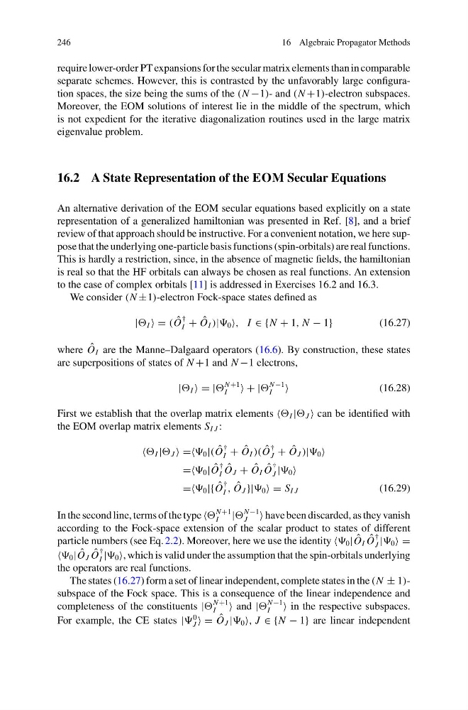
246
16 Algebraic Propagator Methods
require lower-order PT expansions for the secular matrix elements than in comparable
separate schemes. However, this is contrasted by the unfavorably large configuration spaces, the size being the sums of the (N −1)- and (N +1)-electron subspaces.
Moreover, the EOM solutions of interest lie in the middle of the spectrum, which
is not expedient for the iterative diagonalization routines used in the large matrix
eigenvalue problem.
16.2 A State Representation of the EOM Secular Equations
An alternative derivation of the EOM secular equations based explicitly on a state
representation of a generalized hamiltonian was presented in Ref. [8], and a brief
review of that approach should be instructive. For a convenient notation, we here suppose that the underlying one-particle basis functions (spin-orbitals) are real functions.
This is hardly a restriction, since, in the absence of magnetic fields, the hamiltonian
is real so that the HF orbitals can always be chosen as real functions. An extension
to the case of complex orbitals [11] is addressed in Exercises 16.2 and 16.3.
We consider (N ±1)-electron Fock-space states defined as
| I = ( ˆ
O
†
I + ˆ
O I )| 0 , I ∈ {N + 1, N − 1}
(16.27)
where ˆ
O I are the Manne–Dalgaard operators (16.6). By construction, these states
are superpositions of states of N +1 and N −1 electrons,
| I = |
N +1
I
+ |
N −1
I
(16.28)
First we establish that the overlap matrix elements I | J can be identified with
the EOM overlap matrix elements S I J :
I | J == 0 |( ˆ
O
†
I + ˆ
O I )( ˆ
O
†
J + ˆ
O J )| 0
== 0 | ˆ
O
†
I
ˆ
O J + ˆ
O I ˆ
O
†
J | 0
== 0 |{ ˆ
O
†
I , ˆ
O J }| 0 = S I J
(16.29)
In the second line, terms of the type
N +1
I
|
N −1
J
have been discarded, as they vanish
according to the Fock-space extension of the scalar product to states of different
particle numbers (see Eq. 2.2). Moreover, here we use the identity 0 | ˆ
O I ˆ
O
†
J | 0 =
0 | ˆ
O J ˆ
O
†
I | 0 , which is valid under the assumption that the spin-orbitals underlying
the operators are real functions.
The states (16.27) form a set of linear independent, complete states in the (N ± 1)subspace of the Fock space. This is a consequence of the linear independence and
completeness of the constituents |
N +1
I
and |
N −1
I
in the respective subspaces.
For example, the CE states |
0
J = ˆ
O J | 0 , J ∈ {N − 1} are linear independent
16 Algebraic Propagator Methods
require lower-order PT expansions for the secular matrix elements than in comparable
separate schemes. However, this is contrasted by the unfavorably large configuration spaces, the size being the sums of the (N −1)- and (N +1)-electron subspaces.
Moreover, the EOM solutions of interest lie in the middle of the spectrum, which
is not expedient for the iterative diagonalization routines used in the large matrix
eigenvalue problem.
16.2 A State Representation of the EOM Secular Equations
An alternative derivation of the EOM secular equations based explicitly on a state
representation of a generalized hamiltonian was presented in Ref. [8], and a brief
review of that approach should be instructive. For a convenient notation, we here suppose that the underlying one-particle basis functions (spin-orbitals) are real functions.
This is hardly a restriction, since, in the absence of magnetic fields, the hamiltonian
is real so that the HF orbitals can always be chosen as real functions. An extension
to the case of complex orbitals [11] is addressed in Exercises 16.2 and 16.3.
We consider (N ±1)-electron Fock-space states defined as
| I = ( ˆ
O
†
I + ˆ
O I )| 0 , I ∈ {N + 1, N − 1}
(16.27)
where ˆ
O I are the Manne–Dalgaard operators (16.6). By construction, these states
are superpositions of states of N +1 and N −1 electrons,
| I = |
N +1
I
+ |
N −1
I
(16.28)
First we establish that the overlap matrix elements I | J can be identified with
the EOM overlap matrix elements S I J :
I | J == 0 |( ˆ
O
†
I + ˆ
O I )( ˆ
O
†
J + ˆ
O J )| 0
== 0 | ˆ
O
†
I
ˆ
O J + ˆ
O I ˆ
O
†
J | 0
== 0 |{ ˆ
O
†
I , ˆ
O J }| 0 = S I J
(16.29)
In the second line, terms of the type
N +1
I
|
N −1
J
have been discarded, as they vanish
according to the Fock-space extension of the scalar product to states of different
particle numbers (see Eq. 2.2). Moreover, here we use the identity 0 | ˆ
O I ˆ
O
†
J | 0 =
0 | ˆ
O J ˆ
O
†
I | 0 , which is valid under the assumption that the spin-orbitals underlying
the operators are real functions.
The states (16.27) form a set of linear independent, complete states in the (N ± 1)subspace of the Fock space. This is a consequence of the linear independence and
completeness of the constituents |
N +1
I
and |
N −1
I
in the respective subspaces.
For example, the CE states |
0
J = ˆ
O J | 0 , J ∈ {N − 1} are linear independent