

14.3 Properties of the ISR-ADC Schemes
215
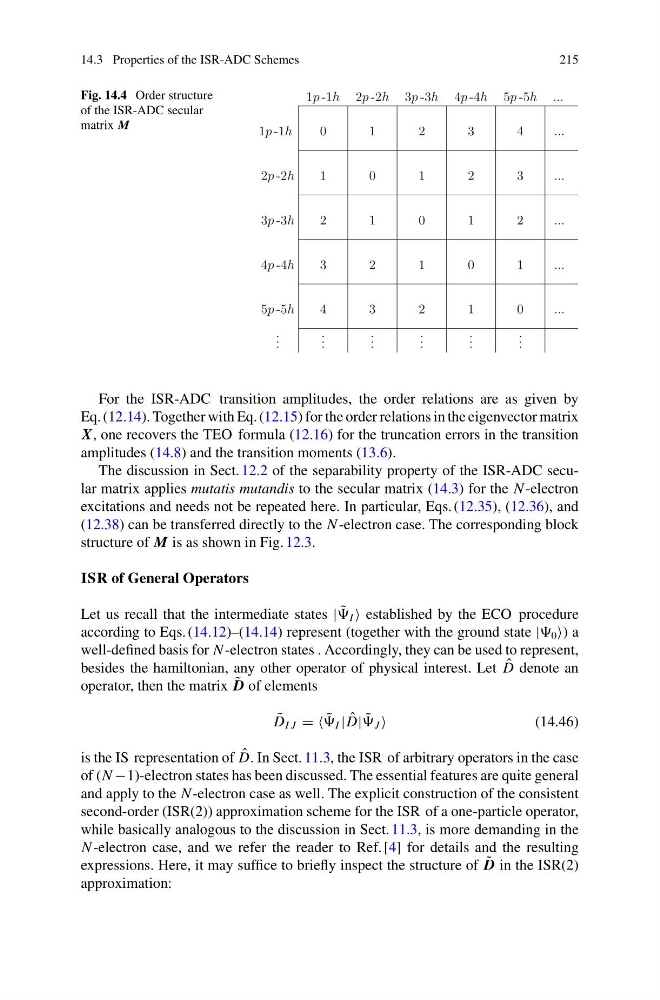
Fig. 14.4 Order structure
of the ISR-ADC secular
matrix M
1p -1h 2p -2h 3p -3h 4p -4h 5p -5h ...
1p -1h
0
1
2
3
4
...
2p -2h
1
0
1
2
3
...
3p -3h
2
1
0
1
2
...
4p -4h
3
2
1
0
1
...
5p -5h
4
3
2
1
0
...
. . .
. . .
. . .
. . .
. . .
. . .
For the ISR-ADC transition amplitudes, the order relations are as given by
Eq. (12.14). Together with Eq. (12.15) for the order relations in the eigenvector matrix
X, one recovers the TEO formula (12.16) for the truncation errors in the transition
amplitudes (14.8) and the transition moments (13.6).
The discussion in Sect. 12.2 of the separability property of the ISR-ADC secular matrix applies mutatis mutandis to the secular matrix (14.3) for the N -electron
excitations and needs not be repeated here. In particular, Eqs. (12.35), (12.36), and
(12.38) can be transferred directly to the N -electron case. The corresponding block
structure of M is as shown in Fig. 12.3.
ISR of General Operators
Let us recall that the intermediate states | ˜
I established by the ECO procedure
according to Eqs. (14.12)–(14.14) represent (together with the ground state | 0 ) a
well-defined basis for N -electron states . Accordingly, they can be used to represent,
besides the hamiltonian, any other operator of physical interest. Let ˆ
D denote an
operator, then the matrix ˜
D of elements
˜
D I J = = ˜
I | ˆ
D| ˜
J
(14.46)
is the IS representation of ˆ
D. In Sect. 11.3, the ISR of arbitrary operators in the case
of (N −1)-electron states has been discussed. The essential features are quite general
and apply to the N -electron case as well. The explicit construction of the consistent
second-order (ISR(2)) approximation scheme for the ISR of a one-particle operator,
while basically analogous to the discussion in Sect. 11.3, is more demanding in the
N -electron case, and we refer the reader to Ref. [4] for details and the resulting
expressions. Here, it may suffice to briefly inspect the structure of ˜
D in the ISR(2)
approximation:
215
Fig. 14.4 Order structure
of the ISR-ADC secular
matrix M
1p -1h 2p -2h 3p -3h 4p -4h 5p -5h ...
1p -1h
0
1
2
3
4
...
2p -2h
1
0
1
2
3
...
3p -3h
2
1
0
1
2
...
4p -4h
3
2
1
0
1
...
5p -5h
4
3
2
1
0
...
. . .
. . .
. . .
. . .
. . .
. . .
For the ISR-ADC transition amplitudes, the order relations are as given by
Eq. (12.14). Together with Eq. (12.15) for the order relations in the eigenvector matrix
X, one recovers the TEO formula (12.16) for the truncation errors in the transition
amplitudes (14.8) and the transition moments (13.6).
The discussion in Sect. 12.2 of the separability property of the ISR-ADC secular matrix applies mutatis mutandis to the secular matrix (14.3) for the N -electron
excitations and needs not be repeated here. In particular, Eqs. (12.35), (12.36), and
(12.38) can be transferred directly to the N -electron case. The corresponding block
structure of M is as shown in Fig. 12.3.
ISR of General Operators
Let us recall that the intermediate states | ˜
I established by the ECO procedure
according to Eqs. (14.12)–(14.14) represent (together with the ground state | 0 ) a
well-defined basis for N -electron states . Accordingly, they can be used to represent,
besides the hamiltonian, any other operator of physical interest. Let ˆ
D denote an
operator, then the matrix ˜
D of elements
˜
D I J = = ˜
I | ˆ
D| ˜
J
(14.46)
is the IS representation of ˆ
D. In Sect. 11.3, the ISR of arbitrary operators in the case
of (N −1)-electron states has been discussed. The essential features are quite general
and apply to the N -electron case as well. The explicit construction of the consistent
second-order (ISR(2)) approximation scheme for the ISR of a one-particle operator,
while basically analogous to the discussion in Sect. 11.3, is more demanding in the
N -electron case, and we refer the reader to Ref. [4] for details and the resulting
expressions. Here, it may suffice to briefly inspect the structure of ˜
D in the ISR(2)
approximation: