

206
14 ADC and ISR Approaches to the Polarization Propagator
f I,rs = = ˜
I |c
†
r c s | 0
(14.4)
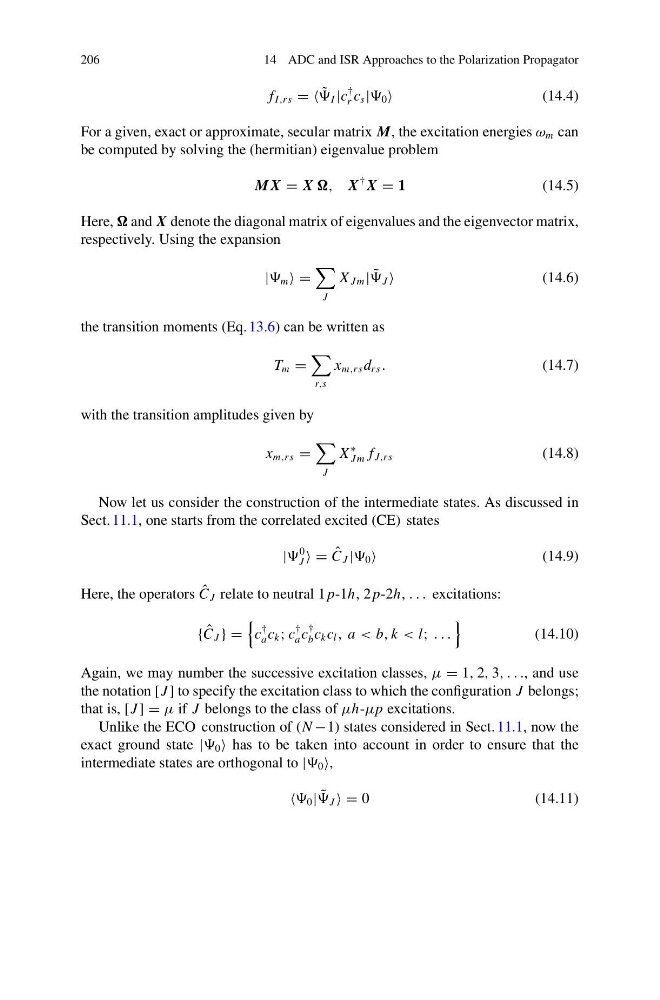
For a given, exact or approximate, secular matrix M, the excitation energies ω m can
be computed by solving the (hermitian) eigenvalue problem
M X = X , X
† X = 1
(14.5)
Here, and X denote the diagonal matrix of eigenvalues and the eigenvector matrix,
respectively. Using the expansion
| m =
J
X J m | ˜
J
(14.6)
the transition moments (Eq. 13.6) can be written as
T m =
r,s
x m,rs d rs .
(14.7)
with the transition amplitudes given by
x m,rs =
J
X
∗
J m f J,rs
(14.8)
Now let us consider the construction of the intermediate states. As discussed in
Sect. 11.1, one starts from the correlated excited (CE) states
|
0
J = ˆ
C J | 0
(14.9)
Here, the operators ˆ
C J relate to neutral 1 p-1h, 2p-2h, . . . excitations:
{ ˆ
C J } =
c
†
a c k ; c
†
a c
†
b c k c l , a < b, k < l; . . .
(14.10)
Again, we may number the successive excitation classes, μ = 1, 2, 3, . . ., and use
the notation [J ] to specify the excitation class to which the configuration J belongs;
that is, [J ] = μ if J belongs to the class of μh-μp excitations.
Unlike the ECO construction of (N −1) states considered in Sect. 11.1, now the
exact ground state | 0 has to be taken into account in order to ensure that the
intermediate states are orthogonal to | 0 ,
0 | ˜
J = 0
(14.11)
14 ADC and ISR Approaches to the Polarization Propagator
f I,rs = = ˜
I |c
†
r c s | 0
(14.4)
For a given, exact or approximate, secular matrix M, the excitation energies ω m can
be computed by solving the (hermitian) eigenvalue problem
M X = X , X
† X = 1
(14.5)
Here, and X denote the diagonal matrix of eigenvalues and the eigenvector matrix,
respectively. Using the expansion
| m =
J
X J m | ˜
J
(14.6)
the transition moments (Eq. 13.6) can be written as
T m =
r,s
x m,rs d rs .
(14.7)
with the transition amplitudes given by
x m,rs =
J
X
∗
J m f J,rs
(14.8)
Now let us consider the construction of the intermediate states. As discussed in
Sect. 11.1, one starts from the correlated excited (CE) states
|
0
J = ˆ
C J | 0
(14.9)
Here, the operators ˆ
C J relate to neutral 1 p-1h, 2p-2h, . . . excitations:
{ ˆ
C J } =
c
†
a c k ; c
†
a c
†
b c k c l , a < b, k < l; . . .
(14.10)
Again, we may number the successive excitation classes, μ = 1, 2, 3, . . ., and use
the notation [J ] to specify the excitation class to which the configuration J belongs;
that is, [J ] = μ if J belongs to the class of μh-μp excitations.
Unlike the ECO construction of (N −1) states considered in Sect. 11.1, now the
exact ground state | 0 has to be taken into account in order to ensure that the
intermediate states are orthogonal to | 0 ,
0 | ˜
J = 0
(14.11)