

13.2 Diagrammatic Perturbation Theory for the Polarization Propagator
203
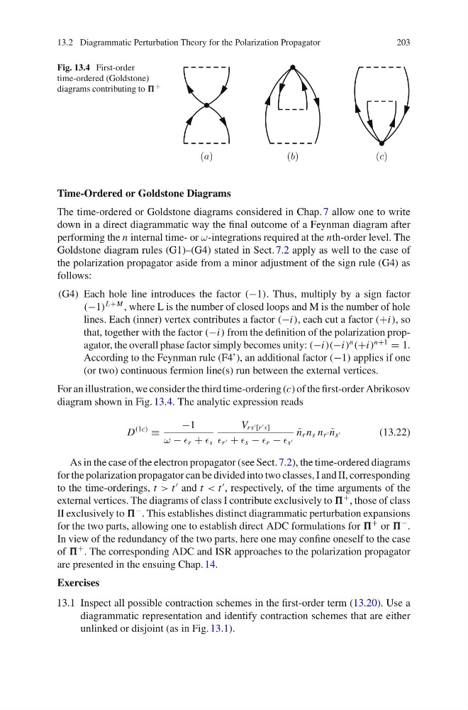
Fig. 13.4 First-order
time-ordered (Goldstone)
diagrams contributing to +
(a)
( b)
( c)
Time-Ordered or Goldstone Diagrams
The time-ordered or Goldstone diagrams considered in Chap. 7 allow one to write
down in a direct diagrammatic way the final outcome of a Feynman diagram after
performing the n internal time- or ω-integrations required at the nth-order level. The
Goldstone diagram rules (G1)–(G4) stated in Sect. 7.2 apply as well to the case of
the polarization propagator aside from a minor adjustment of the sign rule (G4) as
follows:
(G4) Each hole line introduces the factor (−1). Thus, multiply by a sign factor
(−1)
L+M , where L is the number of closed loops and M is the number of hole
lines. Each (inner) vertex contributes a factor (−i), each cut a factor (+i), so
that, together with the factor (−i) from the definition of the polarization propagator, the overall phase factor simply becomes unity: (−i)(−i)
n
(+i)
n+1
= 1.
According to the Feynman rule (F4’), an additional factor (−1) applies if one
(or two) continuous fermion line(s) run between the external vertices.
For an illustration, we consider the third time-ordering (c) of the first-order Abrikosov
diagram shown in Fig. 13.4. The analytic expression reads
D
(1c)
≡
−1
ω − r + s
V rs [r s]
r + s − r − s
¯
n r n s n r ¯
n s
(13.22)
As in the case of the electron propagator (see Sect. 7.2), the time-ordered diagrams
for the polarization propagator can be divided into two classes, I and II, corresponding
to the time-orderings, t > t
and t < t
, respectively, of the time arguments of the
external vertices. The diagrams of class I contribute exclusively to
+ , those of class
II exclusively to
− . This establishes distinct diagrammatic perturbation expansions
for the two parts, allowing one to establish direct ADC formulations for
+ or
− .
In view of the redundancy of the two parts, here one may confine oneself to the case
of
+ . The corresponding ADC and ISR approaches to the polarization propagator
are presented in the ensuing Chap. 14.
Exercises
13.1 Inspect all possible contraction schemes in the first-order term (13.20). Use a
diagrammatic representation and identify contraction schemes that are either
unlinked or disjoint (as in Fig. 13.1).
203
Fig. 13.4 First-order
time-ordered (Goldstone)
diagrams contributing to +
(a)
( b)
( c)
Time-Ordered or Goldstone Diagrams
The time-ordered or Goldstone diagrams considered in Chap. 7 allow one to write
down in a direct diagrammatic way the final outcome of a Feynman diagram after
performing the n internal time- or ω-integrations required at the nth-order level. The
Goldstone diagram rules (G1)–(G4) stated in Sect. 7.2 apply as well to the case of
the polarization propagator aside from a minor adjustment of the sign rule (G4) as
follows:
(G4) Each hole line introduces the factor (−1). Thus, multiply by a sign factor
(−1)
L+M , where L is the number of closed loops and M is the number of hole
lines. Each (inner) vertex contributes a factor (−i), each cut a factor (+i), so
that, together with the factor (−i) from the definition of the polarization propagator, the overall phase factor simply becomes unity: (−i)(−i)
n
(+i)
n+1
= 1.
According to the Feynman rule (F4’), an additional factor (−1) applies if one
(or two) continuous fermion line(s) run between the external vertices.
For an illustration, we consider the third time-ordering (c) of the first-order Abrikosov
diagram shown in Fig. 13.4. The analytic expression reads
D
(1c)
≡
−1
ω − r + s
V rs [r s]
r + s − r − s
¯
n r n s n r ¯
n s
(13.22)
As in the case of the electron propagator (see Sect. 7.2), the time-ordered diagrams
for the polarization propagator can be divided into two classes, I and II, corresponding
to the time-orderings, t > t
and t < t
, respectively, of the time arguments of the
external vertices. The diagrams of class I contribute exclusively to
+ , those of class
II exclusively to
− . This establishes distinct diagrammatic perturbation expansions
for the two parts, allowing one to establish direct ADC formulations for
+ or
− .
In view of the redundancy of the two parts, here one may confine oneself to the case
of
+ . The corresponding ADC and ISR approaches to the polarization propagator
are presented in the ensuing Chap. 14.
Exercises
13.1 Inspect all possible contraction schemes in the first-order term (13.20). Use a
diagrammatic representation and identify contraction schemes that are either
unlinked or disjoint (as in Fig. 13.1).