

202
13 Polarization Propagator
0
1
2A
2B
2C
2D
2E
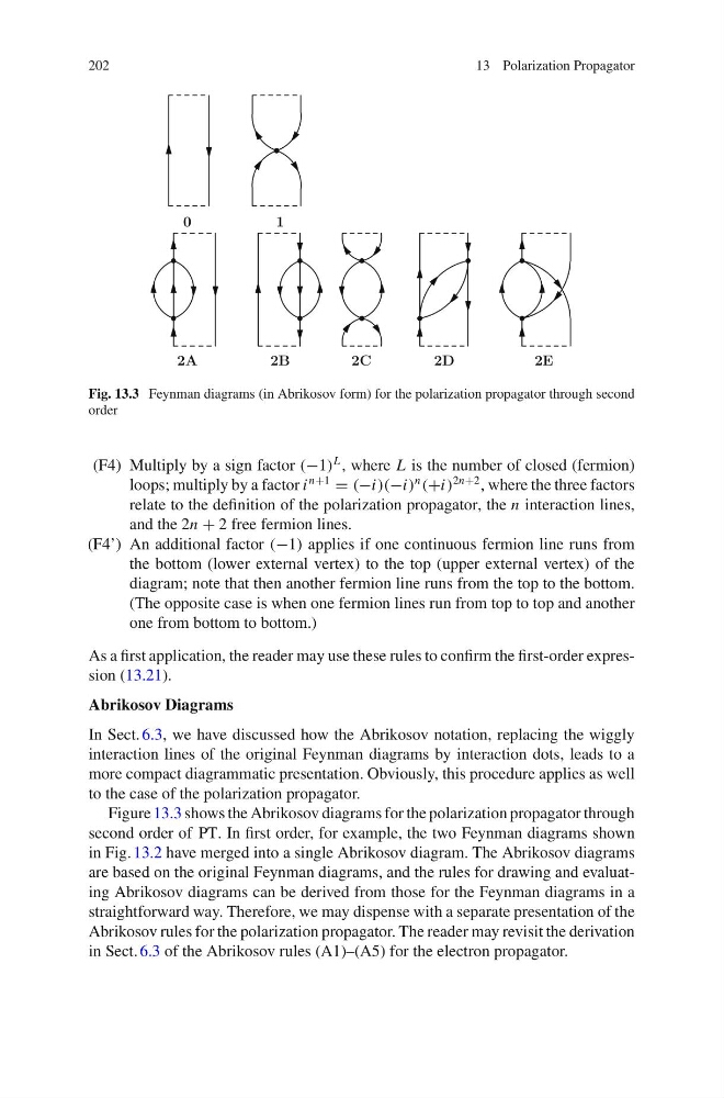
Fig. 13.3 Feynman diagrams (in Abrikosov form) for the polarization propagator through second
order
(F4) Multiply by a sign factor (−1)
L , where L is the number of closed (fermion)
loops; multiply by a factor i
n+1
= (−i)(−i)
n
(+i)
2n+2 , where the three factors
relate to the definition of the polarization propagator, the n interaction lines,
and the 2n + 2 free fermion lines.
(F4’) An additional factor (−1) applies if one continuous fermion line runs from
the bottom (lower external vertex) to the top (upper external vertex) of the
diagram; note that then another fermion line runs from the top to the bottom.
(The opposite case is when one fermion lines run from top to top and another
one from bottom to bottom.)
As a first application, the reader may use these rules to confirm the first-order expression (13.21).
Abrikosov Diagrams
In Sect. 6.3, we have discussed how the Abrikosov notation, replacing the wiggly
interaction lines of the original Feynman diagrams by interaction dots, leads to a
more compact diagrammatic presentation. Obviously, this procedure applies as well
to the case of the polarization propagator.
Figure 13.3 shows the Abrikosov diagrams for the polarization propagator through
second order of PT. In first order, for example, the two Feynman diagrams shown
in Fig. 13.2 have merged into a single Abrikosov diagram. The Abrikosov diagrams
are based on the original Feynman diagrams, and the rules for drawing and evaluating Abrikosov diagrams can be derived from those for the Feynman diagrams in a
straightforward way. Therefore, we may dispense with a separate presentation of the
Abrikosov rules for the polarization propagator. The reader may revisit the derivation
in Sect. 6.3 of the Abrikosov rules (A1)–(A5) for the electron propagator.
13 Polarization Propagator
0
1
2A
2B
2C
2D
2E
Fig. 13.3 Feynman diagrams (in Abrikosov form) for the polarization propagator through second
order
(F4) Multiply by a sign factor (−1)
L , where L is the number of closed (fermion)
loops; multiply by a factor i
n+1
= (−i)(−i)
n
(+i)
2n+2 , where the three factors
relate to the definition of the polarization propagator, the n interaction lines,
and the 2n + 2 free fermion lines.
(F4’) An additional factor (−1) applies if one continuous fermion line runs from
the bottom (lower external vertex) to the top (upper external vertex) of the
diagram; note that then another fermion line runs from the top to the bottom.
(The opposite case is when one fermion lines run from top to top and another
one from bottom to bottom.)
As a first application, the reader may use these rules to confirm the first-order expression (13.21).
Abrikosov Diagrams
In Sect. 6.3, we have discussed how the Abrikosov notation, replacing the wiggly
interaction lines of the original Feynman diagrams by interaction dots, leads to a
more compact diagrammatic presentation. Obviously, this procedure applies as well
to the case of the polarization propagator.
Figure 13.3 shows the Abrikosov diagrams for the polarization propagator through
second order of PT. In first order, for example, the two Feynman diagrams shown
in Fig. 13.2 have merged into a single Abrikosov diagram. The Abrikosov diagrams
are based on the original Feynman diagrams, and the rules for drawing and evaluating Abrikosov diagrams can be derived from those for the Feynman diagrams in a
straightforward way. Therefore, we may dispense with a separate presentation of the
Abrikosov rules for the polarization propagator. The reader may revisit the derivation
in Sect. 6.3 of the Abrikosov rules (A1)–(A5) for the electron propagator.