

200
13 Polarization Propagator
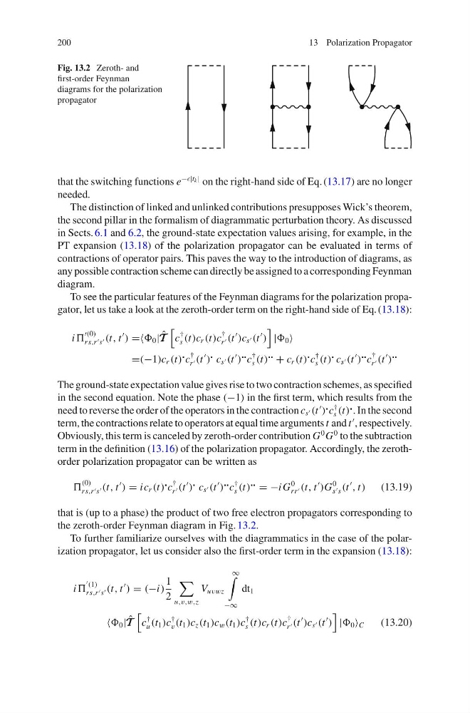
Fig. 13.2 Zeroth- and
first-order Feynman
diagrams for the polarization
propagator
that the switching functions e
−|t k | on the right-hand side of Eq. (13.17) are no longer
needed.
The distinction of linked and unlinked contributions presupposes Wick’s theorem,
the second pillar in the formalism of diagrammatic perturbation theory. As discussed
in Sects. 6.1 and 6.2, the ground-state expectation values arising, for example, in the
PT expansion (13.18) of the polarization propagator can be evaluated in terms of
contractions of operator pairs. This paves the way to the introduction of diagrams, as
any possible contraction scheme can directly be assigned to a corresponding Feynman
diagram.
To see the particular features of the Feynman diagrams for the polarization propagator, let us take a look at the zeroth-order term on the right-hand side of Eq. (13.18):
i
(0)
rs,r s (t, t
) == 0 | ˆ
T T T
c
†
s (t)c r (t)c
†
r (t
)c s (t
)
| 0
=(−1)c r (t)
c
†
r (t
)
c s (t
)
c
†
s (t)
+ c r (t)
c
†
s (t)
c s (t
)
c
†
r (t
)
The ground-state expectation value gives rise to two contraction schemes, as specified
in the second equation. Note the phase (−1) in the first term, which results from the
need to reverse the order of the operators in the contraction c s (t
)
c
†
s (t)
. In the second
term, the contractions relate to operators at equal time arguments t and t
, respectively.
Obviously, this term is canceled by zeroth-order contribution G
0 G
0 to the subtraction
term in the definition (13.16) of the polarization propagator. Accordingly, the zerothorder polarization propagator can be written as
(0)
rs,r s (t, t
) = ic r (t)
c
†
r (t
)
c s (t
)
c
†
s (t)
= −i G
0
rr (t, t
)G
0
s s (t
, t) (13.19)
that is (up to a phase) the product of two free electron propagators corresponding to
the zeroth-order Feynman diagram in Fig. 13.2.
To further familiarize ourselves with the diagrammatics in the case of the polarization propagator, let us consider also the first-order term in the expansion (13.18):
i
(1)
rs,r s (t, t
) = (−i)
1
2
u,v,w,z
V uvwz
∞
−∞
dt 1
0 | ˆ
T T T
c
†
u (t 1 )c
†
v (t 1 )c z (t 1 )c w (t 1 )c
†
s (t)c r (t)c
†
r (t
)c s (t
)
| 0 C
(13.20)
13 Polarization Propagator
Fig. 13.2 Zeroth- and
first-order Feynman
diagrams for the polarization
propagator
that the switching functions e
−|t k | on the right-hand side of Eq. (13.17) are no longer
needed.
The distinction of linked and unlinked contributions presupposes Wick’s theorem,
the second pillar in the formalism of diagrammatic perturbation theory. As discussed
in Sects. 6.1 and 6.2, the ground-state expectation values arising, for example, in the
PT expansion (13.18) of the polarization propagator can be evaluated in terms of
contractions of operator pairs. This paves the way to the introduction of diagrams, as
any possible contraction scheme can directly be assigned to a corresponding Feynman
diagram.
To see the particular features of the Feynman diagrams for the polarization propagator, let us take a look at the zeroth-order term on the right-hand side of Eq. (13.18):
i
(0)
rs,r s (t, t
) == 0 | ˆ
T T T
c
†
s (t)c r (t)c
†
r (t
)c s (t
)
| 0
=(−1)c r (t)
c
†
r (t
)
c s (t
)
c
†
s (t)
+ c r (t)
c
†
s (t)
c s (t
)
c
†
r (t
)
The ground-state expectation value gives rise to two contraction schemes, as specified
in the second equation. Note the phase (−1) in the first term, which results from the
need to reverse the order of the operators in the contraction c s (t
)
c
†
s (t)
. In the second
term, the contractions relate to operators at equal time arguments t and t
, respectively.
Obviously, this term is canceled by zeroth-order contribution G
0 G
0 to the subtraction
term in the definition (13.16) of the polarization propagator. Accordingly, the zerothorder polarization propagator can be written as
(0)
rs,r s (t, t
) = ic r (t)
c
†
r (t
)
c s (t
)
c
†
s (t)
= −i G
0
rr (t, t
)G
0
s s (t
, t) (13.19)
that is (up to a phase) the product of two free electron propagators corresponding to
the zeroth-order Feynman diagram in Fig. 13.2.
To further familiarize ourselves with the diagrammatics in the case of the polarization propagator, let us consider also the first-order term in the expansion (13.18):
i
(1)
rs,r s (t, t
) = (−i)
1
2
u,v,w,z
V uvwz
∞
−∞
dt 1
0 | ˆ
T T T
c
†
u (t 1 )c
†
v (t 1 )c z (t 1 )c w (t 1 )c
†
s (t)c r (t)c
†
r (t
)c s (t
)
| 0 C
(13.20)