

13.2 Diagrammatic Perturbation Theory for the Polarization Propagator
199
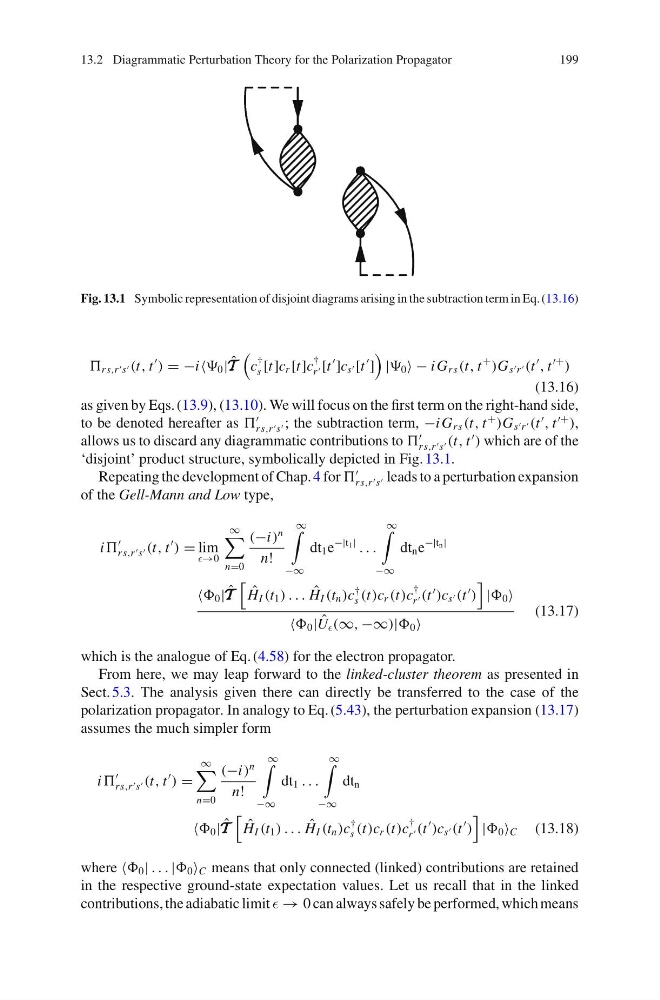
Fig. 13.1 Symbolic representation of disjoint diagrams arising in the subtraction term in Eq. (13.16)
rs,r s (t, t
) = −i 0 | ˆ
T T T
c
†
s [t]c r [t]c
†
r [t
]c s [t
]
| 0 − i G rs (t, t
+
)G s r (t
, t
+
)
(13.16)
as given by Eqs. (13.9), (13.10). We will focus on the first term on the right-hand side,
to be denoted hereafter as
rs,r s ; the subtraction term, −i G rs (t, t
+
)G s r (t
, t
+
),
allows us to discard any diagrammatic contributions to
rs,r s (t, t
) which are of the
‘disjoint’ product structure, symbolically depicted in Fig. 13.1.
Repeating the development of Chap. 4 for
rs,r s leads to a perturbation expansion
of the Gell-Mann and Low type,
i
rs,r s (t, t
) = lim
→0
∞
n=0
(−i)
n
n!
∞
−∞
dt 1 e
−|t 1 |
. . .
∞
−∞
dt n e
−|t n |
0 | ˆ
T T T
ˆ
H I (t 1 ) . . . ˆ
H I (t n )c
†
s (t)c r (t)c
†
r (t
)c s (t
)
| 0
0 | ˆ
U (∞, −∞)| 0
(13.17)
which is the analogue of Eq. (4.58) for the electron propagator.
From here, we may leap forward to the linked-cluster theorem as presented in
Sect. 5.3. The analysis given there can directly be transferred to the case of the
polarization propagator. In analogy to Eq. (5.43), the perturbation expansion (13.17)
assumes the much simpler form
i
rs,r s (t, t
) =
∞
n=0
(−i)
n
n!
∞
−∞
dt 1 . . .
∞
−∞
dt n
0 | ˆ
T T T
ˆ
H I (t 1 ) . . . ˆ
H I (t n )c
†
s (t)c r (t)c
†
r (t
)c s (t
)
| 0 C (13.18)
where 0 | . . . | 0 C means that only connected (linked) contributions are retained
in the respective ground-state expectation values. Let us recall that in the linked
contributions, the adiabatic limit → 0 can always safely be performed, which means
199
Fig. 13.1 Symbolic representation of disjoint diagrams arising in the subtraction term in Eq. (13.16)
rs,r s (t, t
) = −i 0 | ˆ
T T T
c
†
s [t]c r [t]c
†
r [t
]c s [t
]
| 0 − i G rs (t, t
+
)G s r (t
, t
+
)
(13.16)
as given by Eqs. (13.9), (13.10). We will focus on the first term on the right-hand side,
to be denoted hereafter as
rs,r s ; the subtraction term, −i G rs (t, t
+
)G s r (t
, t
+
),
allows us to discard any diagrammatic contributions to
rs,r s (t, t
) which are of the
‘disjoint’ product structure, symbolically depicted in Fig. 13.1.
Repeating the development of Chap. 4 for
rs,r s leads to a perturbation expansion
of the Gell-Mann and Low type,
i
rs,r s (t, t
) = lim
→0
∞
n=0
(−i)
n
n!
∞
−∞
dt 1 e
−|t 1 |
. . .
∞
−∞
dt n e
−|t n |
0 | ˆ
T T T
ˆ
H I (t 1 ) . . . ˆ
H I (t n )c
†
s (t)c r (t)c
†
r (t
)c s (t
)
| 0
0 | ˆ
U (∞, −∞)| 0
(13.17)
which is the analogue of Eq. (4.58) for the electron propagator.
From here, we may leap forward to the linked-cluster theorem as presented in
Sect. 5.3. The analysis given there can directly be transferred to the case of the
polarization propagator. In analogy to Eq. (5.43), the perturbation expansion (13.17)
assumes the much simpler form
i
rs,r s (t, t
) =
∞
n=0
(−i)
n
n!
∞
−∞
dt 1 . . .
∞
−∞
dt n
0 | ˆ
T T T
ˆ
H I (t 1 ) . . . ˆ
H I (t n )c
†
s (t)c r (t)c
†
r (t
)c s (t
)
| 0 C (13.18)
where 0 | . . . | 0 C means that only connected (linked) contributions are retained
in the respective ground-state expectation values. Let us recall that in the linked
contributions, the adiabatic limit → 0 can always safely be performed, which means