

13.1 Definition and Physical Significance
197
rs,r s (t, t
) =
1
2π
∞
−∞
e
−iω(t−t
)
rs,r s (ω)dω
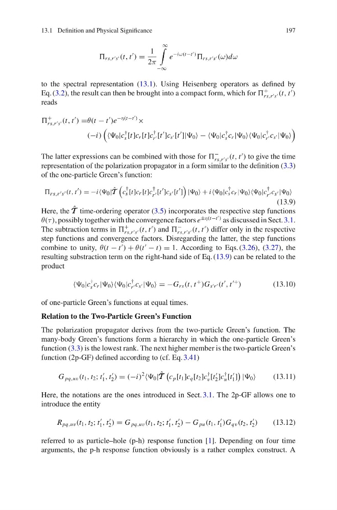
to the spectral representation (13.1). Using Heisenberg operators as defined by
Eq. (3.2), the result can then be brought into a compact form, which for
+
rs,r s (t, t
)
reads
+
rs,r s (t, t
) =θ(t − t
)e
−η(t−t
)
×
(−i)
0 |c
†
s [t]c r [t]c
†
r [t
]c s [t
]| 0 − − 0 |c
†
s c r | 0 0 |c
†
r c s | 0
The latter expressions can be combined with those for
−
rs,r s (t, t
) to give the time
representation of the polarization propagator in a form similar to the definition (3.3)
of the one-particle Green’s function:
rs,r s (t, t ) = −i 0 | ˆ
T T T
c
†
s [t]c r [t]c
†
r [t ]c s [t ]
| 0 + i 0 |c
†
s c r | 0 0 |c
†
r c s | 0
(13.9)
Here, the ˆ
T T T time-ordering operator (3.5) incorporates the respective step functions
θ(τ ), possibly together with the convergence factors e
±η(t−t
) as discussed in Sect. 3.1.
The subtraction terms in
+
rs,r s (t, t
) and
−
rs,r s (t, t
) differ only in the respective
step functions and convergence factors. Disregarding the latter, the step functions
combine to unity, θ(t − t
) + θ(t
− t) = 1. According to Eqs. (3.26), (3.27), the
resulting substraction term on the right-hand side of Eq. (13.9) can be related to the
product
0 |c
†
s c r | 0 0 |c
†
r c s | 0 = −G rs (t, t
+
)G s r (t
, t
+
)
(13.10)
of one-particle Green’s functions at equal times.
Relation to the Two-Particle Green’s Function
The polarization propagator derives from the two-particle Green’s function. The
many-body Green’s functions form a hierarchy in which the one-particle Green’s
function (3.3) is the lowest rank. The next higher member is the two-particle Green’s
function (2p-GF) defined according to (cf. Eq. 3.41)
G pq,uv (t 1 , t 2 ; t
1 , t
2 ) = (−i)
2
0 | ˆ
T T T
c p [t 1 ]c q [t 2 ]c
†
v [t
2 ]c
†
u [t
1 ]
| 0
(13.11)
Here, the notations are the ones introduced in Sect. 3.1. The 2p-GF allows one to
introduce the entity
R pq,uv (t 1 , t 2 ; t
1 , t
2 ) = G pq,uv (t 1 , t 2 ; t
1 , t
2 ) − G pu (t 1 , t
1 )G qv (t 2 , t
2 )
(13.12)
referred to as particle–hole (p-h) response function [1]. Depending on four time
arguments, the p-h response function obviously is a rather complex construct. A
197
rs,r s (t, t
) =
1
2π
∞
−∞
e
−iω(t−t
)
rs,r s (ω)dω
to the spectral representation (13.1). Using Heisenberg operators as defined by
Eq. (3.2), the result can then be brought into a compact form, which for
+
rs,r s (t, t
)
reads
+
rs,r s (t, t
) =θ(t − t
)e
−η(t−t
)
×
(−i)
0 |c
†
s [t]c r [t]c
†
r [t
]c s [t
]| 0 − − 0 |c
†
s c r | 0 0 |c
†
r c s | 0
The latter expressions can be combined with those for
−
rs,r s (t, t
) to give the time
representation of the polarization propagator in a form similar to the definition (3.3)
of the one-particle Green’s function:
rs,r s (t, t ) = −i 0 | ˆ
T T T
c
†
s [t]c r [t]c
†
r [t ]c s [t ]
| 0 + i 0 |c
†
s c r | 0 0 |c
†
r c s | 0
(13.9)
Here, the ˆ
T T T time-ordering operator (3.5) incorporates the respective step functions
θ(τ ), possibly together with the convergence factors e
±η(t−t
) as discussed in Sect. 3.1.
The subtraction terms in
+
rs,r s (t, t
) and
−
rs,r s (t, t
) differ only in the respective
step functions and convergence factors. Disregarding the latter, the step functions
combine to unity, θ(t − t
) + θ(t
− t) = 1. According to Eqs. (3.26), (3.27), the
resulting substraction term on the right-hand side of Eq. (13.9) can be related to the
product
0 |c
†
s c r | 0 0 |c
†
r c s | 0 = −G rs (t, t
+
)G s r (t
, t
+
)
(13.10)
of one-particle Green’s functions at equal times.
Relation to the Two-Particle Green’s Function
The polarization propagator derives from the two-particle Green’s function. The
many-body Green’s functions form a hierarchy in which the one-particle Green’s
function (3.3) is the lowest rank. The next higher member is the two-particle Green’s
function (2p-GF) defined according to (cf. Eq. 3.41)
G pq,uv (t 1 , t 2 ; t
1 , t
2 ) = (−i)
2
0 | ˆ
T T T
c p [t 1 ]c q [t 2 ]c
†
v [t
2 ]c
†
u [t
1 ]
| 0
(13.11)
Here, the notations are the ones introduced in Sect. 3.1. The 2p-GF allows one to
introduce the entity
R pq,uv (t 1 , t 2 ; t
1 , t
2 ) = G pq,uv (t 1 , t 2 ; t
1 , t
2 ) − G pu (t 1 , t
1 )G qv (t 2 , t
2 )
(13.12)
referred to as particle–hole (p-h) response function [1]. Depending on four time
arguments, the p-h response function obviously is a rather complex construct. A