

196
13 Polarization Propagator
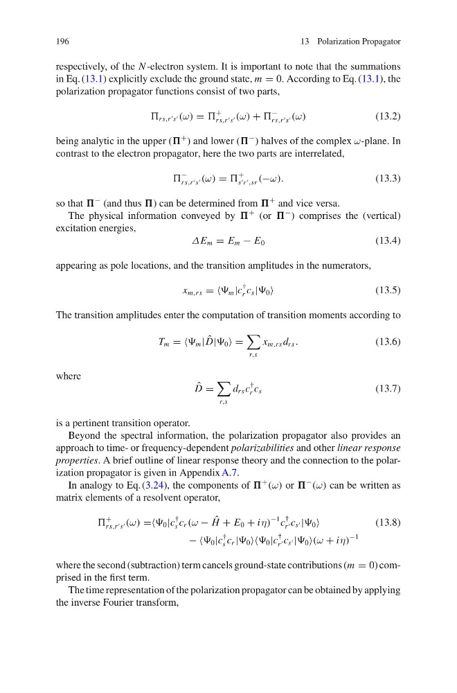
respectively, of the N -electron system. It is important to note that the summations
in Eq. (13.1) explicitly exclude the ground state, m = 0. According to Eq. (13.1), the
polarization propagator functions consist of two parts,
rs,r s (ω) =
+
rs,r s (ω) +
−
rs,r s (ω)
(13.2)
being analytic in the upper (
+ ) and lower (
− ) halves of the complex ω-plane. In
contrast to the electron propagator, here the two parts are interrelated,
−
rs,r s (ω) =
+
s r ,sr (−ω).
(13.3)
so that
− (and thus ) can be determined from
+ and vice versa.
The physical information conveyed by
+ (or
− ) comprises the (vertical)
excitation energies,
ΔE m = E m − E 0
(13.4)
appearing as pole locations, and the transition amplitudes in the numerators,
x m,rs = = m |c
†
r c s | 0
(13.5)
The transition amplitudes enter the computation of transition moments according to
T m = = m | ˆ
D| 0 =
r,s
x m,rs d rs .
(13.6)
where
ˆ
D =
r,s
d rs c
†
r c s
(13.7)
is a pertinent transition operator.
Beyond the spectral information, the polarization propagator also provides an
approach to time- or frequency-dependent polarizabilities and other linear response
properties. A brief outline of linear response theory and the connection to the polarization propagator is given in Appendix A.7.
In analogy to Eq. (3.24), the components of
+
(ω) or
−
(ω) can be written as
matrix elements of a resolvent operator,
+
rs,r s (ω) == 0 |c
†
s c r (ω − ˆ
H + E 0 + iη)
−1 c
†
r c s | 0
(13.8)
− − 0 |c
†
s c r | 0 0 |c
†
r c s | 0 (ω + iη)
−1
where the second (subtraction) term cancels ground-state contributions (m = 0) comprised in the first term.
The time representation of the polarization propagator can be obtained by applying
the inverse Fourier transform,
13 Polarization Propagator
respectively, of the N -electron system. It is important to note that the summations
in Eq. (13.1) explicitly exclude the ground state, m = 0. According to Eq. (13.1), the
polarization propagator functions consist of two parts,
rs,r s (ω) =
+
rs,r s (ω) +
−
rs,r s (ω)
(13.2)
being analytic in the upper (
+ ) and lower (
− ) halves of the complex ω-plane. In
contrast to the electron propagator, here the two parts are interrelated,
−
rs,r s (ω) =
+
s r ,sr (−ω).
(13.3)
so that
− (and thus ) can be determined from
+ and vice versa.
The physical information conveyed by
+ (or
− ) comprises the (vertical)
excitation energies,
ΔE m = E m − E 0
(13.4)
appearing as pole locations, and the transition amplitudes in the numerators,
x m,rs = = m |c
†
r c s | 0
(13.5)
The transition amplitudes enter the computation of transition moments according to
T m = = m | ˆ
D| 0 =
r,s
x m,rs d rs .
(13.6)
where
ˆ
D =
r,s
d rs c
†
r c s
(13.7)
is a pertinent transition operator.
Beyond the spectral information, the polarization propagator also provides an
approach to time- or frequency-dependent polarizabilities and other linear response
properties. A brief outline of linear response theory and the connection to the polarization propagator is given in Appendix A.7.
In analogy to Eq. (3.24), the components of
+
(ω) or
−
(ω) can be written as
matrix elements of a resolvent operator,
+
rs,r s (ω) == 0 |c
†
s c r (ω − ˆ
H + E 0 + iη)
−1 c
†
r c s | 0
(13.8)
− − 0 |c
†
s c r | 0 0 |c
†
r c s | 0 (ω + iη)
−1
where the second (subtraction) term cancels ground-state contributions (m = 0) comprised in the first term.
The time representation of the polarization propagator can be obtained by applying
the inverse Fourier transform,