

12.2 Separability of the ISR-ADC Secular Matrix
183
|
0
J AB
= ˆ
C J AB | 0
= ˆ
C J A |
A
0
ˆ
C J B |
B
0
(12.24)
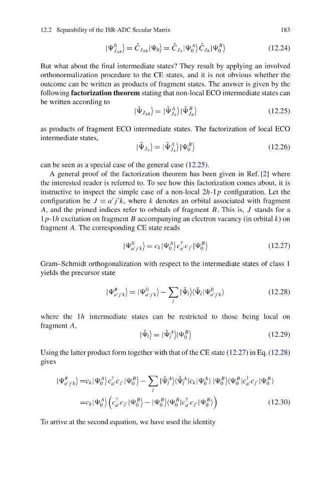
But what about the final intermediate states? They result by applying an involved
orthonormalization procedure to the CE states, and it is not obvious whether the
outcome can be written as products of fragment states. The answer is given by the
following factorization theorem stating that non-local ECO intermediate states can
be written according to
| ˜
J AB
= | ˜
A
J A
| ˜
B
J B
(12.25)
as products of fragment ECO intermediate states. The factorization of local ECO
intermediate states,
| ˜
J A
= | ˜
A
J A
|
B
0
(12.26)
can be seen as a special case of the general case (12.25).
A general proof of the factorization theorem has been given in Ref. [2] where
the interested reader is referred to. To see how this factorization comes about, it is
instructive to inspect the simple case of a non-local 2h-1 p configuration. Let the
configuration be J ≡ a
j
k, where k denotes an orbital associated with fragment
A, and the primed indices refer to orbitals of fragment B. This is, J stands for a
1 p-1h excitation on fragment B accompanying an electron vacancy (in orbital k) on
fragment A. The corresponding CE state reads
|
0
a j k
= c k |
A
0
c
†
a c j |
B
0
(12.27)
Gram–Schmidt orthogonalization with respect to the intermediate states of class 1
yields the precursor state
|
#
a j k
= |
0
a j k
−
l
| ˜
l
˜
l |
0
a j k
(12.28)
where the 1h intermediate states can be restricted to those being local on
fragment A,
| ˜
l
= | ˜
A
l
|
B
0
(12.29)
Using the latter product form together with that of the CE state (12.27) in Eq. (12.28)
gives
|
#
a j k
=c k |
A
0
c
†
a c j |
B
0
−
l
| ˜
A
l
˜
A
l |c k |
A
0 |
B
0
B
0 |c
†
a c j |
B
0
=c k |
A
0
c
†
a c j |
B
0
− |
B
0
B
0 |c
†
a c j |
B
0
(12.30)
To arrive at the second equation, we have used the identity
183
|
0
J AB
= ˆ
C J AB | 0
= ˆ
C J A |
A
0
ˆ
C J B |
B
0
(12.24)
But what about the final intermediate states? They result by applying an involved
orthonormalization procedure to the CE states, and it is not obvious whether the
outcome can be written as products of fragment states. The answer is given by the
following factorization theorem stating that non-local ECO intermediate states can
be written according to
| ˜
J AB
= | ˜
A
J A
| ˜
B
J B
(12.25)
as products of fragment ECO intermediate states. The factorization of local ECO
intermediate states,
| ˜
J A
= | ˜
A
J A
|
B
0
(12.26)
can be seen as a special case of the general case (12.25).
A general proof of the factorization theorem has been given in Ref. [2] where
the interested reader is referred to. To see how this factorization comes about, it is
instructive to inspect the simple case of a non-local 2h-1 p configuration. Let the
configuration be J ≡ a
j
k, where k denotes an orbital associated with fragment
A, and the primed indices refer to orbitals of fragment B. This is, J stands for a
1 p-1h excitation on fragment B accompanying an electron vacancy (in orbital k) on
fragment A. The corresponding CE state reads
|
0
a j k
= c k |
A
0
c
†
a c j |
B
0
(12.27)
Gram–Schmidt orthogonalization with respect to the intermediate states of class 1
yields the precursor state
|
#
a j k
= |
0
a j k
−
l
| ˜
l
˜
l |
0
a j k
(12.28)
where the 1h intermediate states can be restricted to those being local on
fragment A,
| ˜
l
= | ˜
A
l
|
B
0
(12.29)
Using the latter product form together with that of the CE state (12.27) in Eq. (12.28)
gives
|
#
a j k
=c k |
A
0
c
†
a c j |
B
0
−
l
| ˜
A
l
˜
A
l |c k |
A
0 |
B
0
B
0 |c
†
a c j |
B
0
=c k |
A
0
c
†
a c j |
B
0
− |
B
0
B
0 |c
†
a c j |
B
0
(12.30)
To arrive at the second equation, we have used the identity