

9.1 ADC Formulation of the Dynamic Self-Energy Part
139
U
(2)
jab,q ←
1
2
kl
V ab[kl] V kl[q j]
k + l − a − b
(9.17)
Taking also T2(2) into account the full second-order contribution is obtained:
U
(2)
jab,q =
1
2
kl
V ab[kl] V kl[q j]
k + l − a − b
+
ck
V ac[k j] V kb[qc]
a + c − j − k
− (a ↔ b)
(9.18)
To summarize, the ADC(3) secular matrix and U vectors read
(K + C) jab, j a b = (− j + a + b )δ j j δ aa δ bb + C
(1)
jab, j a b
(9.19)
U jab,q = U
(1)
jab,q + U
(2)
jab,q
(9.20)
where C
(1)
jab, j a b is given by Eq. (9.15), and the first- and second-order contributions
to U jab,q by Eqs. (9.10), (9.18). The explicit ADC(3) expressions for both M
+
(ω)
and M
−
(ω) are listed in Appendix A.9.
At the fourth-order level, the ADC procedure is already somewhat elaborate. A
comprehensive presentation has been given in Ref. [3], and we may confine us here to
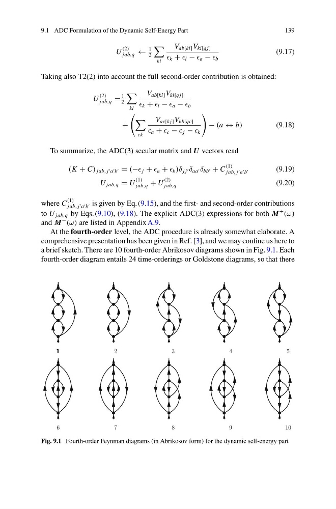
a brief sketch. There are 10 fourth-order Abrikosov diagrams shown in Fig. 9.1. Each
fourth-order diagram entails 24 time-orderings or Goldstone diagrams, so that there
1
Fig. 9.1 Fourth-order Feynman diagrams (in Abrikosov form) for the dynamic self-energy part
139
U
(2)
jab,q ←
1
2
kl
V ab[kl] V kl[q j]
k + l − a − b
(9.17)
Taking also T2(2) into account the full second-order contribution is obtained:
U
(2)
jab,q =
1
2
kl
V ab[kl] V kl[q j]
k + l − a − b
+
ck
V ac[k j] V kb[qc]
a + c − j − k
− (a ↔ b)
(9.18)
To summarize, the ADC(3) secular matrix and U vectors read
(K + C) jab, j a b = (− j + a + b )δ j j δ aa δ bb + C
(1)
jab, j a b
(9.19)
U jab,q = U
(1)
jab,q + U
(2)
jab,q
(9.20)
where C
(1)
jab, j a b is given by Eq. (9.15), and the first- and second-order contributions
to U jab,q by Eqs. (9.10), (9.18). The explicit ADC(3) expressions for both M
+
(ω)
and M
−
(ω) are listed in Appendix A.9.
At the fourth-order level, the ADC procedure is already somewhat elaborate. A
comprehensive presentation has been given in Ref. [3], and we may confine us here to
a brief sketch. There are 10 fourth-order Abrikosov diagrams shown in Fig. 9.1. Each
fourth-order diagram entails 24 time-orderings or Goldstone diagrams, so that there
1
Fig. 9.1 Fourth-order Feynman diagrams (in Abrikosov form) for the dynamic self-energy part