9.1 ADC Formulation of the Dynamic Self-Energy Part
137
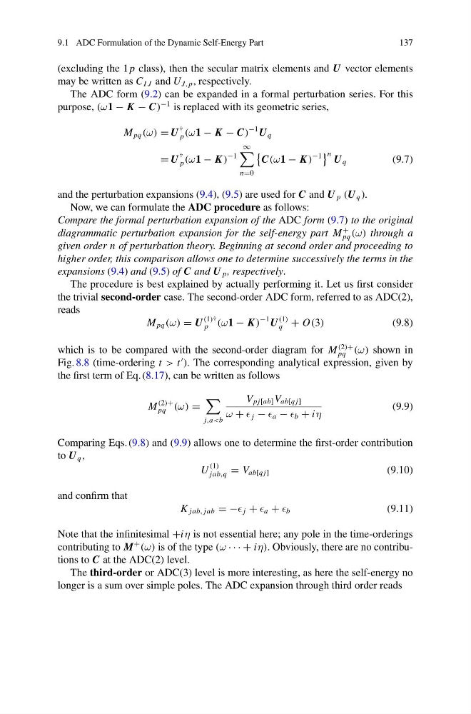
(excluding the 1 p class), then the secular matrix elements and U vector elements
may be written as C I J and U J, p , respectively.
The ADC form (9.2) can be expanded in a formal perturbation series. For this
purpose, (ω1 − K − C)
−1 is replaced with its geometric series,
M pq (ω) = U
†
p (ω1 − K − C)
−1 U q
= U
†
p (ω1 − K )
−1
∞
n=0
C(ω1 − K )
−1
n U q
(9.7)
and the perturbation expansions (9.4), (9.5) are used for C and U p (U q ).
Now, we can formulate the ADC procedure as follows:
Compare the formal perturbation expansion of the ADC form (9.7) to the original
diagrammatic perturbation expansion for the self-energy part M
+
pq (ω) through a
given order n of perturbation theory. Beginning at second order and proceeding to
higher order, this comparison allows one to determine successively the terms in the
expansions (9.4) and (9.5) of C and U p , respectively.
The procedure is best explained by actually performing it. Let us first consider
the trivial second-order case. The second-order ADC form, referred to as ADC(2),
reads
M pq (ω) = U
(1)†
p (ω1 − K )
−1 U
(1)
q + O(3)
(9.8)
which is to be compared with the second-order diagram for M
(2)+
pq (ω) shown in
Fig. 8.8 (time-ordering t > t
). The corresponding analytical expression, given by
the first term of Eq. (8.17), can be written as follows
M
(2)+
pq (ω) =
j,a V pj[ab] V ab[q j]
ω + j − a − b + iη
(9.9)
Comparing Eqs. (9.8) and (9.9) allows one to determine the first-order contribution
to U q ,
U
(1)
jab,q = V ab[q j]
(9.10)
and confirm that
K jab, jab = − j + a + b
(9.11)
Note that the infinitesimal +iη is not essential here; any pole in the time-orderings
contributing to M
+
(ω) is of the type (ω · · · + iη). Obviously, there are no contributions to C at the ADC(2) level.
The third-order or ADC(3) level is more interesting, as here the self-energy no
longer is a sum over simple poles. The ADC expansion through third order reads