

7.2 Performing the Inner Time Integrations
107
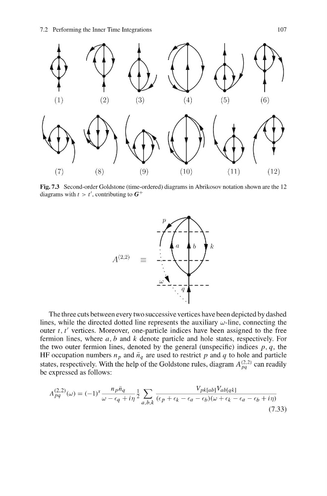
Fig. 7.3 Second-order Goldstone (time-ordered) diagrams in Abrikosov notation shown are the 12
diagrams with t > t , contributing to G
+
The three cuts between every two successive vertices have been depicted by dashed
lines, while the directed dotted line represents the auxiliary ω-line, connecting the
outer t, t
vertices. Moreover, one-particle indices have been assigned to the free
fermion lines, where a, b and k denote particle and hole states, respectively. For
the two outer fermion lines, denoted by the general (unspecific) indices p, q, the
HF occupation numbers n p and ¯
n q are used to restrict p and q to hole and particle
states, respectively. With the help of the Goldstone rules, diagram A
(2,2)
pq can readily
be expressed as follows:
A
(2,2)
pq (ω) = (−1) s
n p ¯
n q
ω − q + iη
1
2
a,b,k
V pk[ab] V ab[qk]
( p + k − a − b )(ω + k − a − b + iη)
(7.33)
107
Fig. 7.3 Second-order Goldstone (time-ordered) diagrams in Abrikosov notation shown are the 12
diagrams with t > t , contributing to G
+
The three cuts between every two successive vertices have been depicted by dashed
lines, while the directed dotted line represents the auxiliary ω-line, connecting the
outer t, t
vertices. Moreover, one-particle indices have been assigned to the free
fermion lines, where a, b and k denote particle and hole states, respectively. For
the two outer fermion lines, denoted by the general (unspecific) indices p, q, the
HF occupation numbers n p and ¯
n q are used to restrict p and q to hole and particle
states, respectively. With the help of the Goldstone rules, diagram A
(2,2)
pq can readily
be expressed as follows:
A
(2,2)
pq (ω) = (−1) s
n p ¯
n q
ω − q + iη
1
2
a,b,k
V pk[ab] V ab[qk]
( p + k − a − b )(ω + k − a − b + iη)
(7.33)