

configuration can be represented more clearly by the polarizability surfaces. As an
example, Fig. 4.7 shows such surfaces for the complex O 2 –Ar. The polarizability
surfaces for other complexes under consideration have analogous shape. It is
obvious, that at θ = 0 and 90° these surfaces are degenerated into the dynamic
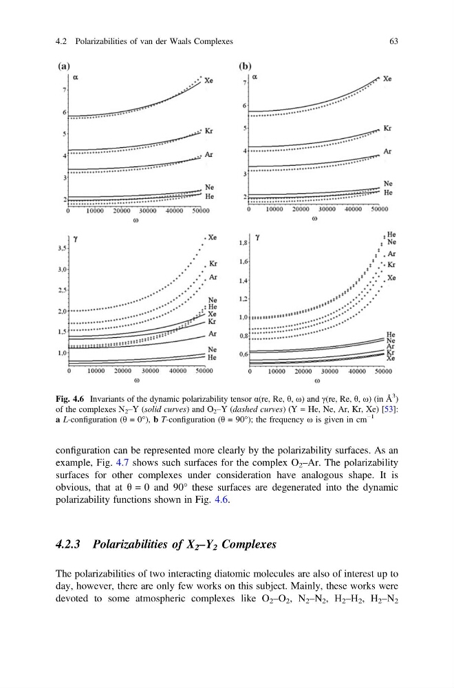
polarizability functions shown in Fig. 4.6.
4.2.3 Polarizabilities of X 2 –Y 2 Complexes
The polarizabilities of two interacting diatomic molecules are also of interest up to
day, however, there are only few works on this subject. Mainly, these works were
devoted to some atmospheric complexes like O 2 –O 2 , N 2 –N 2 , H 2 –H 2 , H 2 –N 2
Fig. 4.6 Invariants of the dynamic polarizability tensor α(re, Re, θ, ω) and γ(re, Re, θ, ω) (in Å
3
)
of the complexes N 2 –Y (solid curves) and O 2 –Y (dashed curves) (Y = He, Ne, Ar, Kr, Xe) [53]:
a L-configuration (θ = 0°), b T-configuration (θ = 90°); the frequency ω is given in cm
−1
4.2 Polarizabilities of van der Waals Complexes
63
example, Fig. 4.7 shows such surfaces for the complex O 2 –Ar. The polarizability
surfaces for other complexes under consideration have analogous shape. It is
obvious, that at θ = 0 and 90° these surfaces are degenerated into the dynamic
polarizability functions shown in Fig. 4.6.
4.2.3 Polarizabilities of X 2 –Y 2 Complexes
The polarizabilities of two interacting diatomic molecules are also of interest up to
day, however, there are only few works on this subject. Mainly, these works were
devoted to some atmospheric complexes like O 2 –O 2 , N 2 –N 2 , H 2 –H 2 , H 2 –N 2
Fig. 4.6 Invariants of the dynamic polarizability tensor α(re, Re, θ, ω) and γ(re, Re, θ, ω) (in Å
3
)
of the complexes N 2 –Y (solid curves) and O 2 –Y (dashed curves) (Y = He, Ne, Ar, Kr, Xe) [53]:
a L-configuration (θ = 0°), b T-configuration (θ = 90°); the frequency ω is given in cm
−1
4.2 Polarizabilities of van der Waals Complexes
63