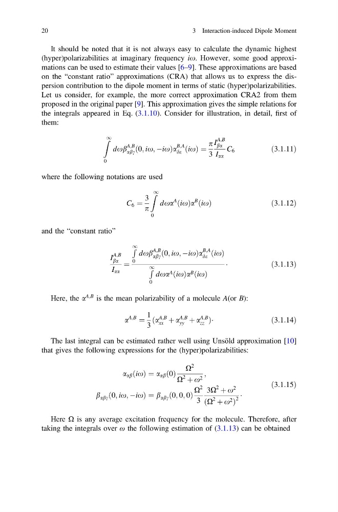
It should be noted that it is not always easy to calculate the dynamic highest
(hyper)polarizabilities at imaginary frequency ix. However, some good approximations can be used to estimate their values [6–9]. These approximations are based
on the “constant ratio” approximations (CRA) that allows us to express the dispersion contribution to the dipole moment in terms of static (hyper)polarizabilities.
Let us consider, for example, the more correct approximation CRA2 from them
proposed in the original paper [9]. This approximation gives the simple relations for
the integrals appeared in Eq. (3.1.10). Consider for illustration, in detail, first of
them:
Z 1
0
dxb
A;B
abc ð0; ix; ÀixÞa
B;A
de ðixÞ ¼
p
3
I
A;B
ba
I aa
C 6
ð3:1:11Þ
where the following notations are used
C 6 ¼
3
p
Z 1
0
dxa
A
ðixÞa
B
ðixÞ
ð 3:1:12Þ
and the “constant ratio”
I
A;B
ba
I aa
¼
R 1
0
dxb
A;B
abc ð0; ix; ÀixÞa
B;A
de ðixÞ
R 1
0
dxa A ðixÞa B ðixÞ
Á
ð 3:1:13Þ
Here, the a
A;B is the mean polarizability of a molecule A(or B):
a
A;B
¼
1
3
ða
A;B
xx þ a
A;B
yy þ a
A;B
zz ÞÁ
ð3:1:14Þ
The last integral can be estimated rather well using Unsöld approximation [10]
that gives the following expressions for the (hyper)polarizabilities:
a ab ðixÞ ¼ a ab 0
ð Þ
X
2
X
2
þ x 2 ;
b abc ð0; ix; ÀixÞ ¼ b abc 0; 0; 0
ð
Þ
X
2
3
3X
2
þ x
2
ðX
2
þ x 2 Þ
2
Á
ð3:1:15Þ
Here Ω is any average excitation frequency for the molecule. Therefore, after
taking the integrals over ω the following estimation of (3.1.13) can be obtained
20
3 Interaction-induced Dipole Moment