

Chapter 3
Interaction-induced Dipole Moment
3.1 General Backgrounds
3.1.1 Computational Features
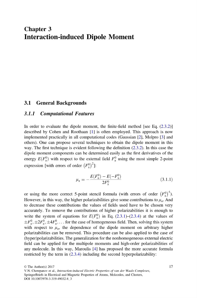
In order to evaluate the dipole moment, the finite-field method [see Eq. (2.3.2)]
described by Cohen and Roothaan [1] is often employed. This approach is now
implemented practically in all computational codes (Gaussian [2], Molpro [3] and
others). One can propose several techniques to obtain the dipole moment in this
way. The first technique is evident following the definition (2.3.2). In this case the
dipole moment components can be determined easily as the first derivatives of the
energy EðF
0
a Þ with respect to the external field F
0
a using the most simple 2-point
expression [with errors of order F
0
a
À Á 2 ]:
l a ¼ À
EðF
0
a Þ À EðÀF
0
a Þ
2F 0
a
ð3:1:1Þ
or using the more correct 5-point stencil formula (with errors of order F
0
a
À Á 4 ).
However, in this way, the higher polarizabilities give some contributions to μ α . And
to decrease these contributions the values of fields used have to be chosen very
accurately. To remove the contributions of higher polarizabilities it is enough to
write the system of equations for EðF
0
a Þ in Eq. (2.3.1)–(2.3.4) at the values of
ÆF
0
a ; Æ2F
0
a ; Æ4F
0
a ; . . . for the case of homogeneous field. Then, solving this system
with respect to μ α , the dependence of the dipole moment on arbitrary higher
polarizabilities can be removed. This procedure can be also applied to the case of
(hyper)polarizabilities. The generalization for the nonhomogeneous external electric
field can be applied for the multipole moments and high-order polarizabilities of
any molecule. In this way, Maroulis [4] has proposed the more accurate formula
restricted by the term in (2.3.4) including the second hyperpolarizability:
© The Author(s) 2017
V.N. Cherepanov et al., Interaction-induced Electric Properties of van der Waals Complexes,
SpringerBriefs in Electrical and Magnetic Properties of Atoms, Molecules, and Clusters,
DOI 10.1007/978-3-319-49032-8_3
17
Interaction-induced Dipole Moment
3.1 General Backgrounds
3.1.1 Computational Features
In order to evaluate the dipole moment, the finite-field method [see Eq. (2.3.2)]
described by Cohen and Roothaan [1] is often employed. This approach is now
implemented practically in all computational codes (Gaussian [2], Molpro [3] and
others). One can propose several techniques to obtain the dipole moment in this
way. The first technique is evident following the definition (2.3.2). In this case the
dipole moment components can be determined easily as the first derivatives of the
energy EðF
0
a Þ with respect to the external field F
0
a using the most simple 2-point
expression [with errors of order F
0
a
À Á 2 ]:
l a ¼ À
EðF
0
a Þ À EðÀF
0
a Þ
2F 0
a
ð3:1:1Þ
or using the more correct 5-point stencil formula (with errors of order F
0
a
À Á 4 ).
However, in this way, the higher polarizabilities give some contributions to μ α . And
to decrease these contributions the values of fields used have to be chosen very
accurately. To remove the contributions of higher polarizabilities it is enough to
write the system of equations for EðF
0
a Þ in Eq. (2.3.1)–(2.3.4) at the values of
ÆF
0
a ; Æ2F
0
a ; Æ4F
0
a ; . . . for the case of homogeneous field. Then, solving this system
with respect to μ α , the dependence of the dipole moment on arbitrary higher
polarizabilities can be removed. This procedure can be also applied to the case of
(hyper)polarizabilities. The generalization for the nonhomogeneous external electric
field can be applied for the multipole moments and high-order polarizabilities of
any molecule. In this way, Maroulis [4] has proposed the more accurate formula
restricted by the term in (2.3.4) including the second hyperpolarizability:
© The Author(s) 2017
V.N. Cherepanov et al., Interaction-induced Electric Properties of van der Waals Complexes,
SpringerBriefs in Electrical and Magnetic Properties of Atoms, Molecules, and Clusters,
DOI 10.1007/978-3-319-49032-8_3
17