

3-5 An Important Identity: 1 bonding electron
41
1
2
ab
ab
*
*
ab
ab
(1) (2)
{ (1) (2) –
(1) (2)} { (1) (2) (1) (2)} / 2
(1) (2)
(12)
1
2
{ (1) (2)
{a(1)b(2) – b(1)a(2)} { (1) (2) (1) (2)} / 2
(1) (2)
(13)
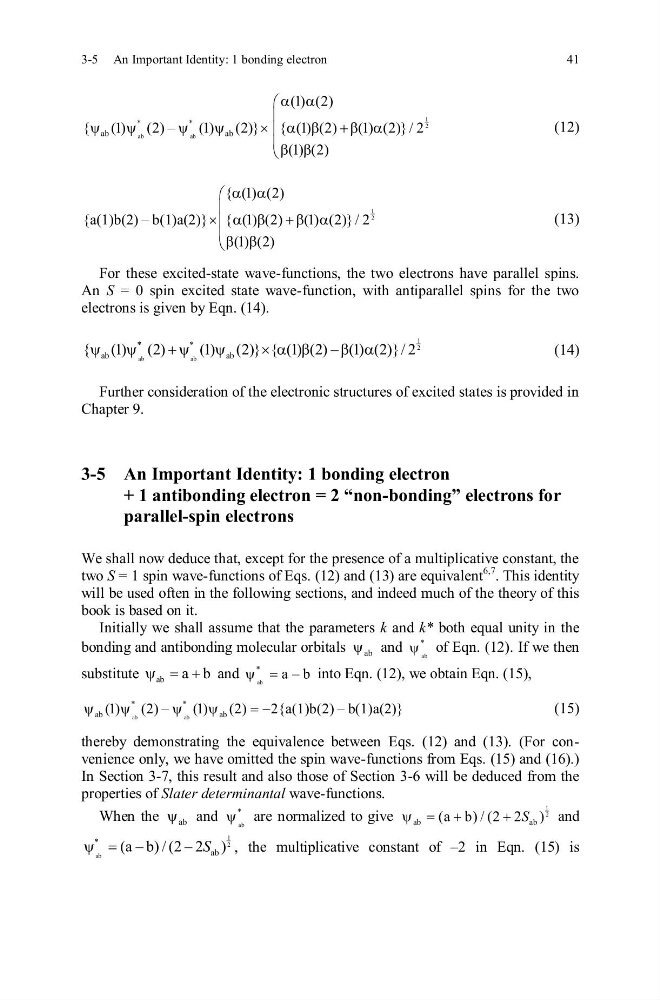
For these excited-state wave-functions, the two electrons have parallel spins.
An S = 0 spin excited state wave-function, with antiparallel spins for the two
electrons is given by Eqn. (14).
1
2
ab
ab
*
*
ab
ab
{ (1) (2)
(1) (2)} { (1) (2) – (1) (2)} / 2
(14)
Further consideration of the electronic structures of excited states is provided in
Chapter 9.
3-5 An Important Identity: 1 bonding electron
+ 1 antibonding electron = 2 “non-bonding” electrons for
parallel-spin electrons
We shall now deduce that, except for the presence of a multiplicative constant, the
two S = 1 spin wave-functions of Eqs. (12) and (13) are equivalent
6,7
. This identity
will be used often in the following sections, and indeed much of the theory of this
book is based on it.
Initially we shall assume that the parameters k and k* both equal unity in the
bonding and antibonding molecular orbitals ab
and
ab
*
of Eqn. (12). If we then
substitute ab a b
and
ab
*
a – b
into Eqn. (12), we obtain Eqn. (15),
ab
ab
*
*
ab
ab
(1) (2) –
(1) (2)
2{a(1)b(2) – b(1)a(2)}
(15)
thereby demonstrating the equivalence between Eqs. (12) and (13). (For convenience only, we have omitted the spin wave-functions from Eqs. (15) and (16).)
In Section 3-7, this result and also those of Section 3-6 will be deduced from the
properties of Slater determinantal wave-functions.
When the ab
and
ab
*
are normalized to give
1
2
ab
ab
(a b) / (2 2 )
S
and
1
2
ab
*
ab
(a – b) / (2 – 2 )
S
, the multiplicative constant of –2 in Eqn. (15) is
41
1
2
ab
ab
*
*
ab
ab
(1) (2)
{ (1) (2) –
(1) (2)} { (1) (2) (1) (2)} / 2
(1) (2)
(12)
1
2
{ (1) (2)
{a(1)b(2) – b(1)a(2)} { (1) (2) (1) (2)} / 2
(1) (2)
(13)
For these excited-state wave-functions, the two electrons have parallel spins.
An S = 0 spin excited state wave-function, with antiparallel spins for the two
electrons is given by Eqn. (14).
1
2
ab
ab
*
*
ab
ab
{ (1) (2)
(1) (2)} { (1) (2) – (1) (2)} / 2
(14)
Further consideration of the electronic structures of excited states is provided in
Chapter 9.
3-5 An Important Identity: 1 bonding electron
+ 1 antibonding electron = 2 “non-bonding” electrons for
parallel-spin electrons
We shall now deduce that, except for the presence of a multiplicative constant, the
two S = 1 spin wave-functions of Eqs. (12) and (13) are equivalent
6,7
. This identity
will be used often in the following sections, and indeed much of the theory of this
book is based on it.
Initially we shall assume that the parameters k and k* both equal unity in the
bonding and antibonding molecular orbitals ab
and
ab
*
of Eqn. (12). If we then
substitute ab a b
and
ab
*
a – b
into Eqn. (12), we obtain Eqn. (15),
ab
ab
*
*
ab
ab
(1) (2) –
(1) (2)
2{a(1)b(2) – b(1)a(2)}
(15)
thereby demonstrating the equivalence between Eqs. (12) and (13). (For convenience only, we have omitted the spin wave-functions from Eqs. (15) and (16).)
In Section 3-7, this result and also those of Section 3-6 will be deduced from the
properties of Slater determinantal wave-functions.
When the ab
and
ab
*
are normalized to give
1
2
ab
ab
(a b) / (2 2 )
S
and
1
2
ab
*
ab
(a – b) / (2 – 2 )
S
, the multiplicative constant of –2 in Eqn. (15) is