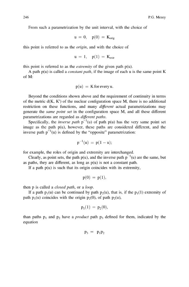
From such a parametrization by the unit interval, with the choice of
u ¼ 0; p 0
ð Þ ¼ K orig
this point is referred to as the origin, and with the choice of
u ¼ 1; p 1
ð Þ ¼ K extr
this point is referred to as the extremity of the given path p(u).
A path p(u) is called a constant path, if the image of each u is the same point K
of M:
p u
ð Þ ¼ K for every u:
Beyond the conditions shown above and the requirement of continuity in terms
of the metric d(K, K′) of the nuclear configuration space M, there is no additional
restriction on these functions, and many different actual parametrizations may
generate the same point set in the configuration space M, and all these different
parametrizations are regarded as different paths.
Specifically, the inverse path p
−1 (u) of path p(u) has the very same point set
image as the path p(u), however, these paths are considered different, and the
inverse path p
−1 (u) is defined by the “opposite” parametrization:
p
À1 u
ð Þ ¼ p 1 À u
ð
Þ;
for example, the roles of origin and extremity are interchanged.
Clearly, as point sets, the path p(u), and the inverse path p
−1 (u) are the same, but
as paths, they are different, as long as p(u) is not a constant path.
If a path p(u) is such that its origin coincides with its extremity,
p 0
ð Þ ¼ p 1
ð Þ;
then p is called a closed path, or a loop.
If a path p 1 (u) can be continued by path p 2 (u), that is, if the p 1 (1) extremity of
path p 1 (u) coincides with the origin p 2 (0), of path p 2 (u),
p 1 1
ð Þ ¼ p 2 0
ð Þ;
than paths p 1 and p 2 have a product path p 3 defined for them, indicated by the
equation
p 3 ¼ p 1 p 2
246
P.G. Mezey