

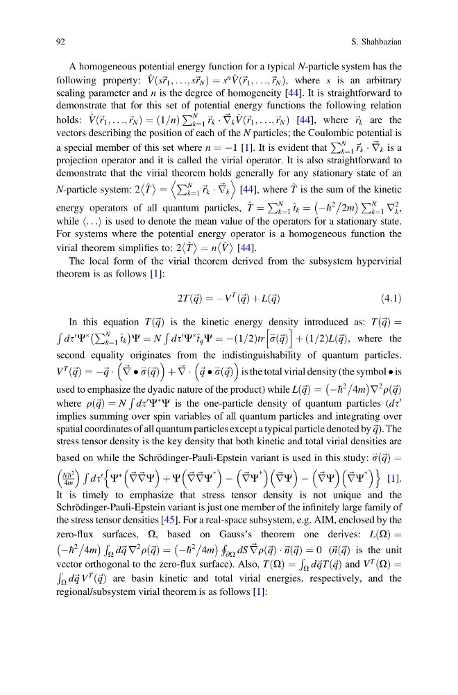
A homogeneous potential energy function for a typical N-particle system has the
following property: ^
V s~ r 1 ; . . .; s~ r N
ð
Þ¼s
n ^
V ~ r 1 ; . . .;~ r N
ð
Þ , where s is an arbitrary
scaling parameter and n is the degree of homogeneity [44]. It is straightforward to
demonstrate that for this set of potential energy functions the following relation
holds: ^
V ~ r 1 ; . . .;~ r N
ð
Þ¼ 1=n
ð
Þ
P N
k¼1 ~ r k Á ~
r k ^
V ~ r 1 ; . . .;~ r N
ð
Þ [44], where ~ r k are the
vectors describing the position of each of the N particles; the Coulombic potential is
a special member of this set where n ¼ À1 [1]. It is evident that
P N
k¼1 ~ r k Á ~
r k is a
projection operator and it is called the virial operator. It is also straightforward to
demonstrate that the virial theorem holds generally for any stationary state of an
N-particle system: 2 ^
T
¼
P N
k¼1 ~ r k Á ~
r k
D
E
[44], where ^
T is the sum of the kinetic
energy operators of all quantum particles, ^
T ¼
P N
k¼1
^ t k ¼ À h
2
2m
À
ÁP N
k¼1 r
2
k ,
while . . .
h i is used to denote the mean value of the operators for a stationary state.
For systems where the potential energy operator is a homogeneous function the
virial theorem simplifies to: 2 ^
T
¼ n ^
V
[44].
The local form of the virial theorem derived from the subsystem hypervirial
theorem is as follows [1]:
2T ~ q
ð Þ ¼ ÀV
T
~ q
ð Þ þ L ~ q
ð Þ
ð4:1Þ
In this equation T ~ q
ð Þ is the kinetic energy density introduced as: T ~ q
ð Þ ¼
R
ds
0
W
à P N
k¼1
^ t k
À
Á W ¼ N
R
ds
0
W
à ^ t q W ¼ À 1=2
ð
Þtr r
$ ~ q
ð Þ
h
i
þ 1=2
ð
ÞL ~ q
ð Þ, where the
second equality originates from the indistinguishability of quantum particles.
V
T
~ q
ð Þ ¼ À~ q Á ~
r r
$ ~ q
ð Þ
þ ~
r Á ~ q r
$ ~ q
ð Þ
is the total virial density (the symbol is
used to emphasize the dyadic nature of the product) while L ~ q
ð Þ ¼ À h
2
4m
À
Á r
2
q ~ q
ð Þ
where q ~ q
ð Þ ¼ N
R
ds
0
W
Ã
W is the one-particle density of quantum particles (ds
0
implies summing over spin variables of all quantum particles and integrating over
spatial coordinates of all quantum particles except a typical particle denoted by~ q). The
stress tensor density is the key density that both kinetic and total virial densities are
based on while the Schrödinger-Pauli-Epstein variant is used in this study: r
$ ~ q
ð Þ ¼
N h
2
4m
R
ds
0
W
à ~
r ~
rW
þ W ~
r ~
rW
Ã
À ~
rW
Ã
~
rW
À ~
rW
~
rW
Ã
n
o
[1].
It is timely to emphasize that stress tensor density is not unique and the
Schrödinger-Pauli-Epstein variant is just one member of the infinitely large family of
the stress tensor densities [45]. For a real-space subsystem, e.g. AIM, enclosed by the
zero-flux surfaces, X, based on Gauss’s theorem one derives: L X
ð Þ ¼
À h
2
4m
À
ÁR
X d~ q r
2
q ~ q
ð Þ ¼ À h
2
4m
À
ÁH
@X dS ~
rq ~ q
ð Þ Á~ n ~ q
ð Þ ¼ 0 (~ n ~ q
ð Þ is the unit
vector orthogonal to the zero-flux surface). Also, T X
ð Þ ¼
R
X d~ qT ~ q
ð Þ and V
T
X
ð Þ ¼
R
X d~ q V
T
~ q
ð Þ are basin kinetic and total virial energies, respectively, and the
regional/subsystem virial theorem is as follows [1]:
92
S. Shahbazian
following property: ^
V s~ r 1 ; . . .; s~ r N
ð
Þ¼s
n ^
V ~ r 1 ; . . .;~ r N
ð
Þ , where s is an arbitrary
scaling parameter and n is the degree of homogeneity [44]. It is straightforward to
demonstrate that for this set of potential energy functions the following relation
holds: ^
V ~ r 1 ; . . .;~ r N
ð
Þ¼ 1=n
ð
Þ
P N
k¼1 ~ r k Á ~
r k ^
V ~ r 1 ; . . .;~ r N
ð
Þ [44], where ~ r k are the
vectors describing the position of each of the N particles; the Coulombic potential is
a special member of this set where n ¼ À1 [1]. It is evident that
P N
k¼1 ~ r k Á ~
r k is a
projection operator and it is called the virial operator. It is also straightforward to
demonstrate that the virial theorem holds generally for any stationary state of an
N-particle system: 2 ^
T
¼
P N
k¼1 ~ r k Á ~
r k
D
E
[44], where ^
T is the sum of the kinetic
energy operators of all quantum particles, ^
T ¼
P N
k¼1
^ t k ¼ À h
2
2m
À
ÁP N
k¼1 r
2
k ,
while . . .
h i is used to denote the mean value of the operators for a stationary state.
For systems where the potential energy operator is a homogeneous function the
virial theorem simplifies to: 2 ^
T
¼ n ^
V
[44].
The local form of the virial theorem derived from the subsystem hypervirial
theorem is as follows [1]:
2T ~ q
ð Þ ¼ ÀV
T
~ q
ð Þ þ L ~ q
ð Þ
ð4:1Þ
In this equation T ~ q
ð Þ is the kinetic energy density introduced as: T ~ q
ð Þ ¼
R
ds
0
W
à P N
k¼1
^ t k
À
Á W ¼ N
R
ds
0
W
à ^ t q W ¼ À 1=2
ð
Þtr r
$ ~ q
ð Þ
h
i
þ 1=2
ð
ÞL ~ q
ð Þ, where the
second equality originates from the indistinguishability of quantum particles.
V
T
~ q
ð Þ ¼ À~ q Á ~
r r
$ ~ q
ð Þ
þ ~
r Á ~ q r
$ ~ q
ð Þ
is the total virial density (the symbol is
used to emphasize the dyadic nature of the product) while L ~ q
ð Þ ¼ À h
2
4m
À
Á r
2
q ~ q
ð Þ
where q ~ q
ð Þ ¼ N
R
ds
0
W
Ã
W is the one-particle density of quantum particles (ds
0
implies summing over spin variables of all quantum particles and integrating over
spatial coordinates of all quantum particles except a typical particle denoted by~ q). The
stress tensor density is the key density that both kinetic and total virial densities are
based on while the Schrödinger-Pauli-Epstein variant is used in this study: r
$ ~ q
ð Þ ¼
N h
2
4m
R
ds
0
W
à ~
r ~
rW
þ W ~
r ~
rW
Ã
À ~
rW
Ã
~
rW
À ~
rW
~
rW
Ã
n
o
[1].
It is timely to emphasize that stress tensor density is not unique and the
Schrödinger-Pauli-Epstein variant is just one member of the infinitely large family of
the stress tensor densities [45]. For a real-space subsystem, e.g. AIM, enclosed by the
zero-flux surfaces, X, based on Gauss’s theorem one derives: L X
ð Þ ¼
À h
2
4m
À
ÁR
X d~ q r
2
q ~ q
ð Þ ¼ À h
2
4m
À
ÁH
@X dS ~
rq ~ q
ð Þ Á~ n ~ q
ð Þ ¼ 0 (~ n ~ q
ð Þ is the unit
vector orthogonal to the zero-flux surface). Also, T X
ð Þ ¼
R
X d~ qT ~ q
ð Þ and V
T
X
ð Þ ¼
R
X d~ q V
T
~ q
ð Þ are basin kinetic and total virial energies, respectively, and the
regional/subsystem virial theorem is as follows [1]:
92
S. Shahbazian