

8
A. Monari and X. Assfeld
(1.3)
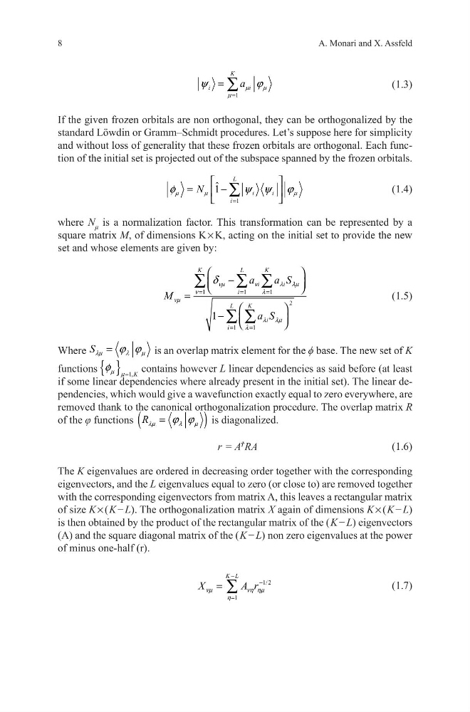
If the given frozen orbitals are non orthogonal, they can be orthogonalized by the
standard Löwdin or Gramm–Schmidt procedures. Let’s suppose here for simplicity
and without loss of generality that these frozen orbitals are orthogonal. Each function of the initial set is projected out of the subspace spanned by the frozen orbitals.
(1.4)
where N μ is a normalization factor. This transformation can be represented by a
square matrix M, of dimensions K × K, acting on the initial set to provide the new
set and whose elements are given by:
(1.5)
Where S λµ
λ
µ
ϕ ϕ
=
is an overlap matrix element for the ϕ base. The new set of K
functions { } 1,K
µ µ
φ = contains however L linear dependencies as said before (at least
if some linear dependencies where already present in the initial set). The linear dependencies, which would give a wavefunction exactly equal to zero everywhere, are
removed thank to the canonical orthogonalization procedure. The overlap matrix R
of the φ functions (
)
R λµ
λ
µ
ϕ ϕ
=
is diagonalized.
(1.6)
The K eigenvalues are ordered in decreasing order together with the corresponding
eigenvectors, and the L eigenvalues equal to zero (or close to) are removed together
with the corresponding eigenvectors from matrix A, this leaves a rectangular matrix
of size K × ( K − L). The orthogonalization matrix X again of dimensions K × ( K − L)
is then obtained by the product of the rectangular matrix of the ( K − L) eigenvectors
(A) and the square diagonal matrix of the ( K − L) non zero eigenvalues at the power
of minus one-half (r).
(1.7)
1
K
i
i
a µ µ
µ
ψ
ϕ
=
= ∑
1
ˆ
1
L
i
i
i
N
µ
µ
µ
φ
ψ ψ ϕ
=
=
-
∑
1
1
1
2
1
1
1
K
L
K
i
i
i
L
K
i
i
a
a S
M
a S
νµ
ν
λ λµ
ν
λ
νµ
λ λµ
λ
δ
=
=
=
=
=
-
=
-
∑
∑ ∑
∑ ∑
r = A
Ϯ
RA
1/ 2
1
K L
X
A r
νµ
νη ηµ
η
-
-
=
= ∑
A. Monari and X. Assfeld
(1.3)
If the given frozen orbitals are non orthogonal, they can be orthogonalized by the
standard Löwdin or Gramm–Schmidt procedures. Let’s suppose here for simplicity
and without loss of generality that these frozen orbitals are orthogonal. Each function of the initial set is projected out of the subspace spanned by the frozen orbitals.
(1.4)
where N μ is a normalization factor. This transformation can be represented by a
square matrix M, of dimensions K × K, acting on the initial set to provide the new
set and whose elements are given by:
(1.5)
Where S λµ
λ
µ
ϕ ϕ
=
is an overlap matrix element for the ϕ base. The new set of K
functions { } 1,K
µ µ
φ = contains however L linear dependencies as said before (at least
if some linear dependencies where already present in the initial set). The linear dependencies, which would give a wavefunction exactly equal to zero everywhere, are
removed thank to the canonical orthogonalization procedure. The overlap matrix R
of the φ functions (
)
R λµ
λ
µ
ϕ ϕ
=
is diagonalized.
(1.6)
The K eigenvalues are ordered in decreasing order together with the corresponding
eigenvectors, and the L eigenvalues equal to zero (or close to) are removed together
with the corresponding eigenvectors from matrix A, this leaves a rectangular matrix
of size K × ( K − L). The orthogonalization matrix X again of dimensions K × ( K − L)
is then obtained by the product of the rectangular matrix of the ( K − L) eigenvectors
(A) and the square diagonal matrix of the ( K − L) non zero eigenvalues at the power
of minus one-half (r).
(1.7)
1
K
i
i
a µ µ
µ
ψ
ϕ
=
= ∑
1
ˆ
1
L
i
i
i
N
µ
µ
µ
φ
ψ ψ ϕ
=
=
-
∑
1
1
1
2
1
1
1
K
L
K
i
i
i
L
K
i
i
a
a S
M
a S
νµ
ν
λ λµ
ν
λ
νµ
λ λµ
λ
δ
=
=
=
=
=
-
=
-
∑
∑ ∑
∑ ∑
r = A
Ϯ
RA
1/ 2
1
K L
X
A r
νµ
νη ηµ
η
-
-
=
= ∑