

160
L. González et al.
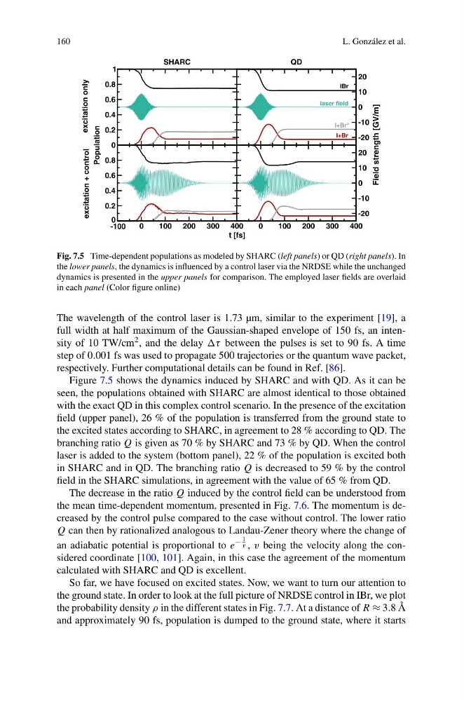
Fig. 7.5 Time-dependent populations as modeled by SHARC (left panels) or QD (right panels). In
the lower panels, the dynamics is influenced by a control laser via the NRDSE while the unchanged
dynamics is presented in the upper panels for comparison. The employed laser fields are overlaid
in each panel (Color figure online)
The wavelength of the control laser is 1.73 µm, similar to the experiment [19], a
full width at half maximum of the Gaussian-shaped envelope of 150 fs, an intensity of 10 TW/cm 2 , and the delay τ between the pulses is set to 90 fs. A time
step of 0.001 fs was used to propagate 500 trajectories or the quantum wave packet,
respectively. Further computational details can be found in Ref. [86].
Figure 7.5 shows the dynamics induced by SHARC and with QD. As it can be
seen, the populations obtained with SHARC are almost identical to those obtained
with the exact QD in this complex control scenario. In the presence of the excitation
field (upper panel), 26 % of the population is transferred from the ground state to
the excited states according to SHARC, in agreement to 28 % according to QD. The
branching ratio Q is given as 70 % by SHARC and 73 % by QD. When the control
laser is added to the system (bottom panel), 22 % of the population is excited both
in SHARC and in QD. The branching ratio Q is decreased to 59 % by the control
field in the SHARC simulations, in agreement with the value of 65 % from QD.
The decrease in the ratio Q induced by the control field can be understood from
the mean time-dependent momentum, presented in Fig. 7.6. The momentum is decreased by the control pulse compared to the case without control. The lower ratio
Q can then by rationalized analogous to Landau-Zener theory where the change of
an adiabatic potential is proportional to e
−
1
v , v being the velocity along the considered coordinate [100, 101]. Again, in this case the agreement of the momentum
calculated with SHARC and QD is excellent.
So far, we have focused on excited states. Now, we want to turn our attention to
the ground state. In order to look at the full picture of NRDSE control in IBr, we plot
the probability density ρ in the different states in Fig. 7.7. At a distance of R ≈ 3.8 Å
and approximately 90 fs, population is dumped to the ground state, where it starts
L. González et al.
Fig. 7.5 Time-dependent populations as modeled by SHARC (left panels) or QD (right panels). In
the lower panels, the dynamics is influenced by a control laser via the NRDSE while the unchanged
dynamics is presented in the upper panels for comparison. The employed laser fields are overlaid
in each panel (Color figure online)
The wavelength of the control laser is 1.73 µm, similar to the experiment [19], a
full width at half maximum of the Gaussian-shaped envelope of 150 fs, an intensity of 10 TW/cm 2 , and the delay τ between the pulses is set to 90 fs. A time
step of 0.001 fs was used to propagate 500 trajectories or the quantum wave packet,
respectively. Further computational details can be found in Ref. [86].
Figure 7.5 shows the dynamics induced by SHARC and with QD. As it can be
seen, the populations obtained with SHARC are almost identical to those obtained
with the exact QD in this complex control scenario. In the presence of the excitation
field (upper panel), 26 % of the population is transferred from the ground state to
the excited states according to SHARC, in agreement to 28 % according to QD. The
branching ratio Q is given as 70 % by SHARC and 73 % by QD. When the control
laser is added to the system (bottom panel), 22 % of the population is excited both
in SHARC and in QD. The branching ratio Q is decreased to 59 % by the control
field in the SHARC simulations, in agreement with the value of 65 % from QD.
The decrease in the ratio Q induced by the control field can be understood from
the mean time-dependent momentum, presented in Fig. 7.6. The momentum is decreased by the control pulse compared to the case without control. The lower ratio
Q can then by rationalized analogous to Landau-Zener theory where the change of
an adiabatic potential is proportional to e
−
1
v , v being the velocity along the considered coordinate [100, 101]. Again, in this case the agreement of the momentum
calculated with SHARC and QD is excellent.
So far, we have focused on excited states. Now, we want to turn our attention to
the ground state. In order to look at the full picture of NRDSE control in IBr, we plot
the probability density ρ in the different states in Fig. 7.7. At a distance of R ≈ 3.8 Å
and approximately 90 fs, population is dumped to the ground state, where it starts